7.3: An Example of Simple Regression

Last updated
Save as PDF

Page ID: 7237

\( \newcommand{\vecs}[1]{\overset { \scriptstyle \rightharpoonup} {\mathbf{#1}} } \) \( \newcommand{\vecd}[1]{\overset{-\!-\!\rightharpoonup}{\vphantom{a}\smash {#1}}} \)\(\newcommand{\id}{\mathrm{id}}\) \( \newcommand{\Span}{\mathrm{span}}\) \( \newcommand{\kernel}{\mathrm{null}\,}\) \( \newcommand{\range}{\mathrm{range}\,}\) \( \newcommand{\RealPart}{\mathrm{Re}}\) \( \newcommand{\ImaginaryPart}{\mathrm{Im}}\) \( \newcommand{\Argument}{\mathrm{Arg}}\) \( \newcommand{\norm}[1]{\| #1 \|}\) \( \newcommand{\inner}[2]{\langle #1, #2 \rangle}\) \( \newcommand{\Span}{\mathrm{span}}\) \(\newcommand{\id}{\mathrm{id}}\) \( \newcommand{\Span}{\mathrm{span}}\) \( \newcommand{\kernel}{\mathrm{null}\,}\) \( \newcommand{\range}{\mathrm{range}\,}\) \( \newcommand{\RealPart}{\mathrm{Re}}\) \( \newcommand{\ImaginaryPart}{\mathrm{Im}}\) \( \newcommand{\Argument}{\mathrm{Arg}}\) \( \newcommand{\norm}[1]{\| #1 \|}\) \( \newcommand{\inner}[2]{\langle #1, #2 \rangle}\) \( \newcommand{\Span}{\mathrm{span}}\)\(\newcommand{\AA}{\unicode[.8,0]{x212B}}\)

The following example uses a measure of peoples’ political ideology to predict their perceptions of the risks posed by global climate change. OLS regression can be done using the lm function in R. For this example, we are again using the class data set.

ols1 <- lm(ds$glbcc_risk~ds$ideol)
summary(ols1)

## 
## Call:
## lm(formula = ds$glbcc_risk ~ ds$ideol)
## 
## Residuals:
##    Min     1Q Median     3Q    Max 
## -8.726 -1.633  0.274  1.459  6.506 
## 
## Coefficients:
##             Estimate Std. Error t value            Pr(>|t|)    
## (Intercept) 10.81866    0.14189   76.25 <0.0000000000000002 ***
## ds$ideol    -1.04635    0.02856  -36.63 <0.0000000000000002 ***
## ---
## Signif. codes:  0 '***' 0.001 '**' 0.01 '*' 0.05 '.' 0.1 ' ' 1
## 
## Residual standard error: 2.479 on 2511 degrees of freedom
##   (34 observations deleted due to missingness)
## Multiple R-squared:  0.3483, Adjusted R-squared:  0.348 
## F-statistic:  1342 on 1 and 2511 DF,  p-value: < 0.00000000000000022

The output in R provides quite a lot of information about the relationship between the measures of ideology and perceived risks of climate change. It provides an overview of the distribution of the residuals; the estimated coefficients for ^αα^ and ^ββ^; the results of hypothesis tests; and overall measures of model fit" – all of which we will discuss in detail in later chapters. For now, note that the estimated BB for ideology is negative, which indicates that as the value for ideology increases—in our data this means more conservative—the perceived risk of climate change decreases. Specifically, for each one-unit increase in the ideology scale, perceived climate change risk decreases by -1.0463463.

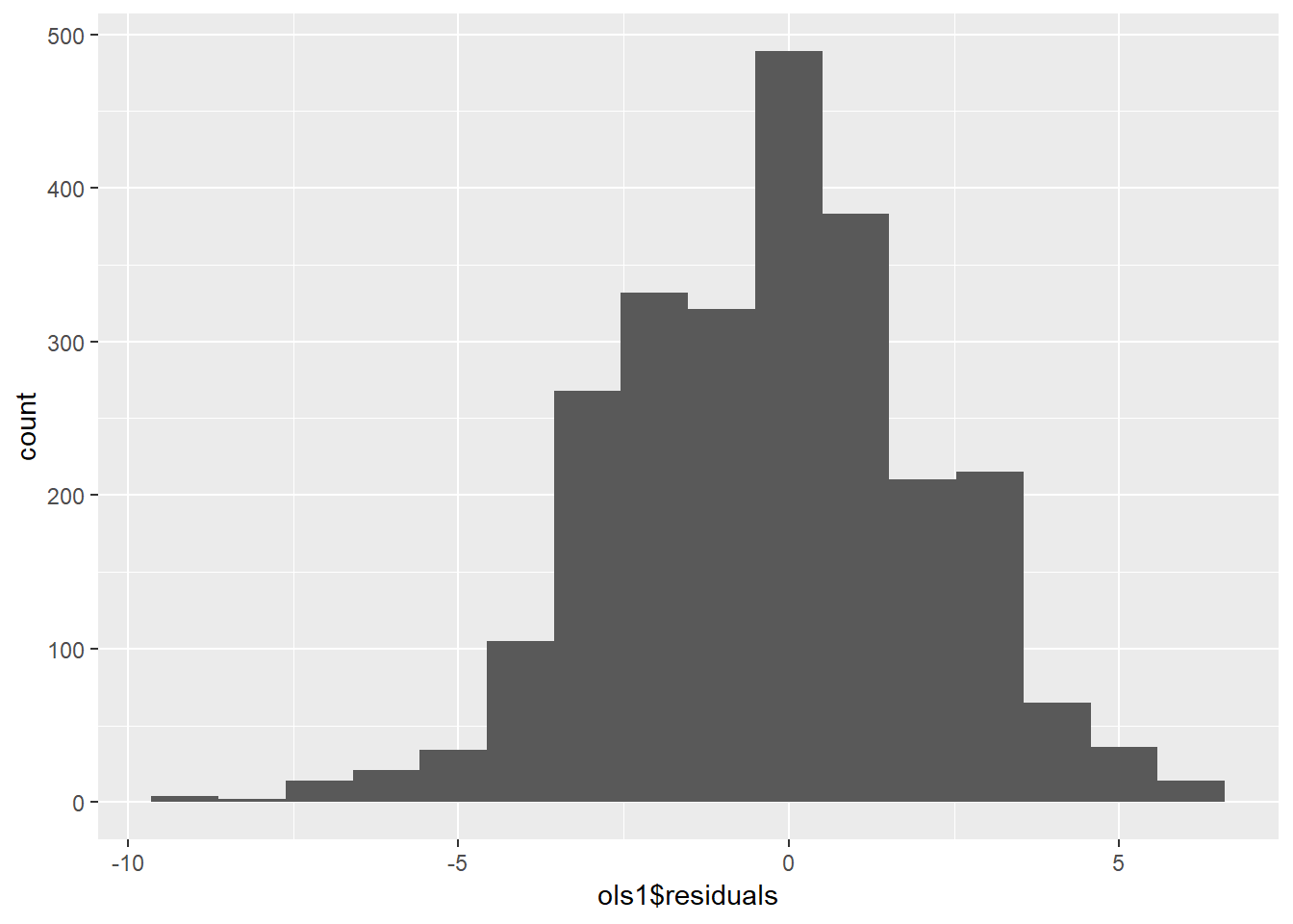
We can also examine the distribution of the residuals, using a histogram and a density curve. This is shown in Figure \(\PageIndex{4}\) and Figure \(\PageIndex{5}\). Note that we will discuss residual diagnostics in detail in future chapters.

data.frame(ols1$residuals) %>%
  ggplot(aes(ols1$residuals)) +
  geom_histogram(bins = 16)

Figure \(\PageIndex{4}\): Residuals of Simple Regression: Histogram

data.frame(ols1$residuals) %>%
  ggplot(aes(ols1$residuals)) +
  geom_density(adjust = 1.5)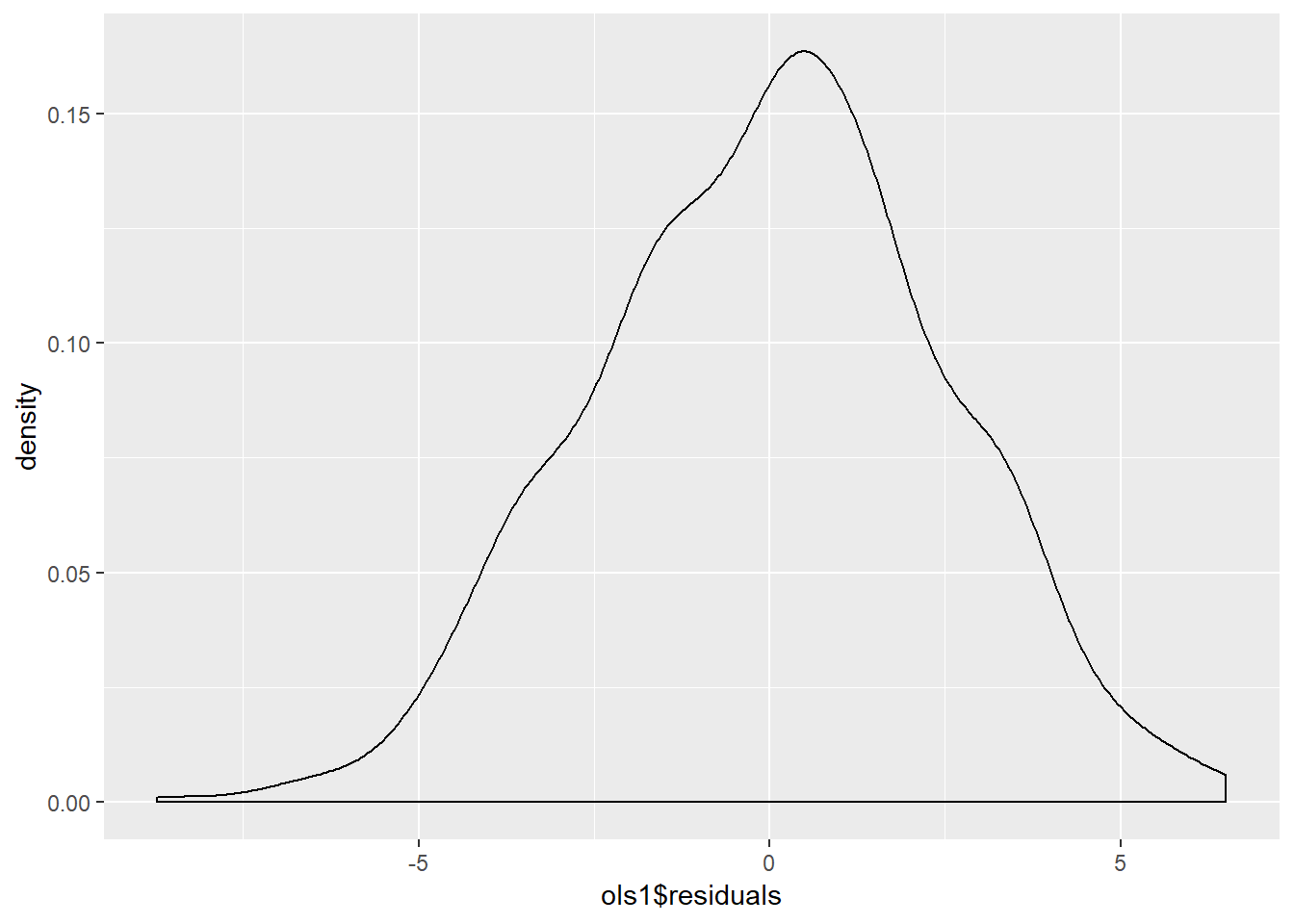

Figure \(\PageIndex{5}\): Residuals of Simple Regression: Density

For purposes of this Chapter, be sure that you can run the basic bivariate OLS regression model in R. If you can – congratulations! If not, try again. And again. And again…

Actually, we assume only that the means of the errors drawn from repeated samples of observations will be normally distributed – but we will deal with that wrinkle later on.↩