6.4: Scatterplots

Last updated
Save as PDF

Page ID: 7233

\( \newcommand{\vecs}[1]{\overset { \scriptstyle \rightharpoonup} {\mathbf{#1}} } \) \( \newcommand{\vecd}[1]{\overset{-\!-\!\rightharpoonup}{\vphantom{a}\smash {#1}}} \)\(\newcommand{\id}{\mathrm{id}}\) \( \newcommand{\Span}{\mathrm{span}}\) \( \newcommand{\kernel}{\mathrm{null}\,}\) \( \newcommand{\range}{\mathrm{range}\,}\) \( \newcommand{\RealPart}{\mathrm{Re}}\) \( \newcommand{\ImaginaryPart}{\mathrm{Im}}\) \( \newcommand{\Argument}{\mathrm{Arg}}\) \( \newcommand{\norm}[1]{\| #1 \|}\) \( \newcommand{\inner}[2]{\langle #1, #2 \rangle}\) \( \newcommand{\Span}{\mathrm{span}}\) \(\newcommand{\id}{\mathrm{id}}\) \( \newcommand{\Span}{\mathrm{span}}\) \( \newcommand{\kernel}{\mathrm{null}\,}\) \( \newcommand{\range}{\mathrm{range}\,}\) \( \newcommand{\RealPart}{\mathrm{Re}}\) \( \newcommand{\ImaginaryPart}{\mathrm{Im}}\) \( \newcommand{\Argument}{\mathrm{Arg}}\) \( \newcommand{\norm}[1]{\| #1 \|}\) \( \newcommand{\inner}[2]{\langle #1, #2 \rangle}\) \( \newcommand{\Span}{\mathrm{span}}\)\(\newcommand{\AA}{\unicode[.8,0]{x212B}}\)

As noted earlier, it is often useful to try and see patterns between two variables. We examined the density plots of males and females with regard to climate change risk, then we tested these differences for statistical significance. However, we often want to know more than the mean difference between groups; we may also want to know if differences exist for variables with several possible values. For example, here we examine the relationship between ideology and perceived risk of climate change. One of the more efficient ways to do this is to produce a scatterplot. %Use geom_jitter. This is because ideology and glbcc risk are discrete variables(i.e., whole numbers), so we need to “jitter” the data. If your values are continuous, use geom_point.¹³ The result is shown in Figure.

ds %>%
  ggplot(aes(ideol, glbcc_risk)) +
  geom_jitter(shape = 1)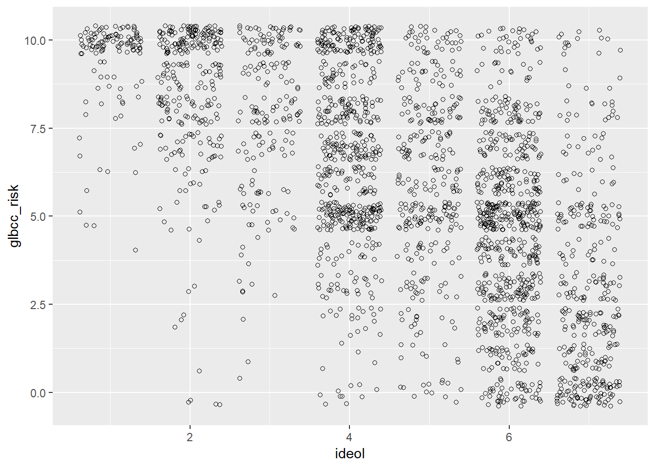

Figure \(\PageIndex{7}\): Scatterplot of Ideology and glbcc Risk

We can see that the density of values indicates that strong liberals—11’s on the ideology scale—tend to view climate change as quite risky, whereas strong conservatives—77’s on the ideology scale—tend to view climate change as less risky. Like our previous example, we want to know more about the nature of this relationship. Therefore, we can plot a regression line and a “loess” line. These lines are the linear and nonlinear estimates of the relationship between political ideology and the perceived risk of climate change. We’ll have more to say about the linear estimates when we turn to regression analysis in the next chapter.

ds %>%
  drop_na(glbcc_risk, ideol) %>%
  ggplot(aes(ideol, glbcc_risk)) +
  geom_jitter(shape = 1) +
  geom_smooth(method = "loess", color = "green") +
  geom_smooth(method = "lm", color = "red")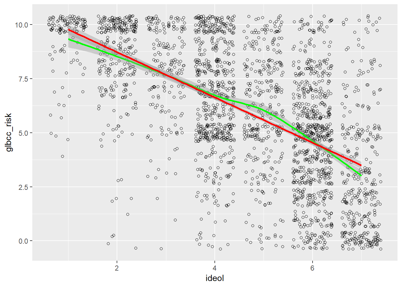

Figure \(\PageIndex{8}\): Scatterplot of Ideology and GLBCC Risk with Regression Line and Lowess Line

Note that the regression lines both slope downward, with average perceived risk ranging from over 8 for the strong liberals (ideology=1) to less than 5 for strong conservatives (ideology=7). This illustrates how scatterplots can provide information about the nature of the relationship between two variables. We will take the next step – to bivariate regression analysis – in the next chapter.

Figure \(\PageIndex{9}\): Chi Square Table

To reiterate the general decision rule: if the probability that we could have a 20% difference in our sample if the null hypothesis is true is less than .05, we will reject our null hypothesis.↩
That means a “jit” (a very small value) is applied to each observed point on the plot, so you can see observations that are “stacked” on the same coordinate. Ha! Just kidding; they’re not called jits. We don’t know what they’re called. But they ought to be called jits.↩