12.3: Multiple Regression Example

Last updated
Save as PDF

Page ID: 7260

\( \newcommand{\vecs}[1]{\overset { \scriptstyle \rightharpoonup} {\mathbf{#1}} } \) \( \newcommand{\vecd}[1]{\overset{-\!-\!\rightharpoonup}{\vphantom{a}\smash {#1}}} \)\(\newcommand{\id}{\mathrm{id}}\) \( \newcommand{\Span}{\mathrm{span}}\) \( \newcommand{\kernel}{\mathrm{null}\,}\) \( \newcommand{\range}{\mathrm{range}\,}\) \( \newcommand{\RealPart}{\mathrm{Re}}\) \( \newcommand{\ImaginaryPart}{\mathrm{Im}}\) \( \newcommand{\Argument}{\mathrm{Arg}}\) \( \newcommand{\norm}[1]{\| #1 \|}\) \( \newcommand{\inner}[2]{\langle #1, #2 \rangle}\) \( \newcommand{\Span}{\mathrm{span}}\) \(\newcommand{\id}{\mathrm{id}}\) \( \newcommand{\Span}{\mathrm{span}}\) \( \newcommand{\kernel}{\mathrm{null}\,}\) \( \newcommand{\range}{\mathrm{range}\,}\) \( \newcommand{\RealPart}{\mathrm{Re}}\) \( \newcommand{\ImaginaryPart}{\mathrm{Im}}\) \( \newcommand{\Argument}{\mathrm{Arg}}\) \( \newcommand{\norm}[1]{\| #1 \|}\) \( \newcommand{\inner}[2]{\langle #1, #2 \rangle}\) \( \newcommand{\Span}{\mathrm{span}}\)\(\newcommand{\AA}{\unicode[.8,0]{x212B}}\)

library(psych)
describe(data.frame(ds.temp$glbcc_risk,ds.temp$ideol,
                    ds.temp$age))

##                    vars    n  mean    sd median trimmed   mad min max
## ds.temp.glbcc_risk    1 2513  5.95  3.07      6    6.14  2.97   0  10
## ds.temp.ideol         2 2513  4.66  1.73      5    4.76  1.48   1   7
## ds.temp.age           3 2513 60.38 14.19     62   61.01 13.34  18  99
##                    range  skew kurtosis   se
## ds.temp.glbcc_risk    10 -0.32    -0.94 0.06
## ds.temp.ideol          6 -0.45    -0.79 0.03
## ds.temp.age           81 -0.38    -0.23 0.28

library(car)
scatterplotMatrix(data.frame(ds.temp$glbcc_risk,
                             ds.temp$ideol,ds.temp$age),
                  diagonal="density")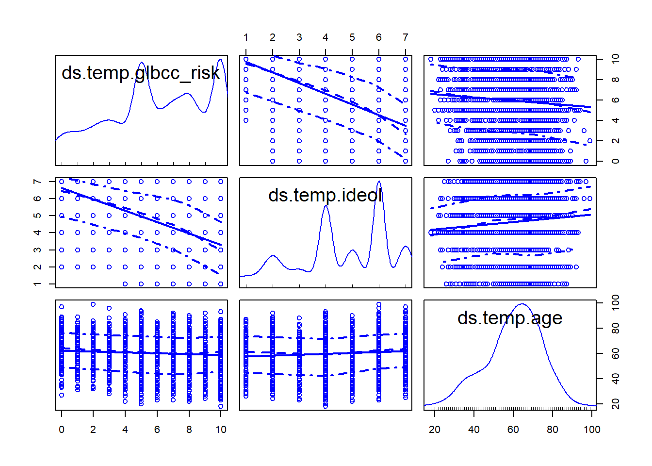

In this section, we walk through another example of multiple regression. First, we start with our two IV model.

ols1 <- lm(glbcc_risk ~ age+ideol, data=ds.temp)
summary(ols1)

## 
## Call:
## lm(formula = glbcc_risk ~ age + ideol, data = ds.temp)
## 
## Residuals:
##     Min      1Q  Median      3Q     Max 
## -8.7913 -1.6252  0.2785  1.4674  6.6075 
## 
## Coefficients:
##              Estimate Std. Error t value            Pr(>|t|)    
## (Intercept) 11.096064   0.244640  45.357 <0.0000000000000002 ***
## age         -0.004872   0.003500  -1.392               0.164    
## ideol       -1.042748   0.028674 -36.366 <0.0000000000000002 ***
## ---
## Signif. codes:  0 '***' 0.001 '**' 0.01 '*' 0.05 '.' 0.1 ' ' 1
## 
## Residual standard error: 2.479 on 2510 degrees of freedom
## Multiple R-squared:  0.3488, Adjusted R-squared:  0.3483 
## F-statistic: 672.2 on 2 and 2510 DF,  p-value: < 0.00000000000000022

The results show that the relationship between age and perceived risk (glbccrsk) is negative and insignificant. The relationship between ideology and perceived risk is negative and significant. The coefficients of the XX’s are interpreted in the same way as with simple regression, except that we are now controlling for the effect of the other XX’s by removing their influence on the estimated coefficient. Therefore, we say that as ideology increases one unit, perceptions of the risk of climate change (glbccrsk) decrease by -1.0427478, controlling for the effect of age.

As was the case with simple regression, multiple regression finds the intercept and slopes that minimize the sum of the squared residuals. With only one IV the relationship can be represented in a two-dimensional plane (a graph) as a line, but each IV adds another dimension. Two IVs create a regression plane within a cube, as shown in Figure \(\PageIndex{3}\). The Figure shows a scatterplot of perceived climate change risk, age, and ideology coupled with the regression plane. Note that this is a sample of 200 observations from the larger data set. Were we to add more IVs, we would generate a hypercube… and we haven’t found a clever way to draw that yet.

ds200 <- ds.temp[sample(1:nrow(ds.temp), 200, replace=FALSE),]
library(scatterplot3d)  
s3d <-scatterplot3d(ds200$age,
                    ds200$ideol,
                    ds200$glbcc_risk
                    ,pch=16, highlight.3d=TRUE,  
type="h", main="3D Scatterplot")
s3d$plane3d(ols1)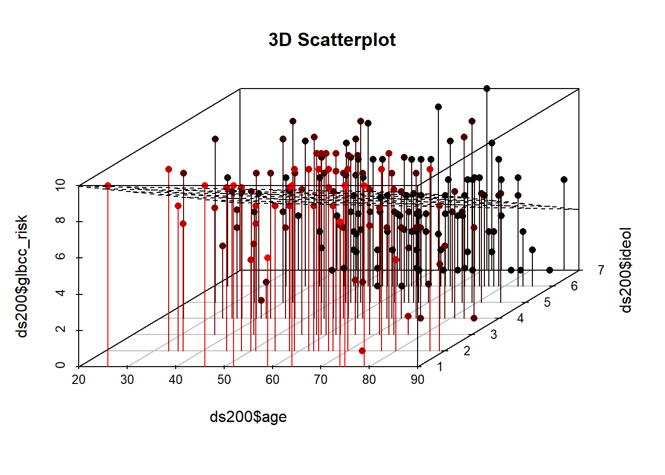

Figure \(\PageIndex{3}\): Scatterplot and Regression Plane of gcc risk, age, and ideology

In the next example education is added to the model.

ds.temp <- filter(ds) %>%
  dplyr::select(glbcc_risk, age, education, income, ideol) %>%
  na.omit()

ols2 <- lm(glbcc_risk ~ age + education + ideol, data = ds.temp)
summary(ols2)

## 
## Call:
## lm(formula = glbcc_risk ~ age + education + ideol, data = ds.temp)
## 
## Residuals:
##     Min      1Q  Median      3Q     Max 
## -8.8092 -1.6355  0.2388  1.4279  6.6334 
## 
## Coefficients:
##              Estimate Std. Error t value            Pr(>|t|)    
## (Intercept) 10.841669   0.308416  35.153 <0.0000000000000002 ***
## age         -0.003246   0.003652  -0.889               0.374    
## education    0.036775   0.028547   1.288               0.198    
## ideol       -1.044827   0.029829 -35.027 <0.0000000000000002 ***
## ---
## Signif. codes:  0 '***' 0.001 '**' 0.01 '*' 0.05 '.' 0.1 ' ' 1
## 
## Residual standard error: 2.437 on 2268 degrees of freedom
## Multiple R-squared:  0.3607, Adjusted R-squared:  0.3598 
## F-statistic: 426.5 on 3 and 2268 DF,  p-value: < 0.00000000000000022

We see that as a respondent’s education increases one unit on the education scale, perceived risk appears to increase by 0.0367752, keeping age and ideology constant. However, this result is not significant. In the final example, income is added to the model. Note that the size and significance of education actually increases once income is included, indicating that education only has bearing on the perceived risks of climate change once the independent effect of income is considered.

options(scipen = 999) #to turn off scientific notation
ols3 <- lm(glbcc_risk ~ age + education + income + ideol, data = ds.temp)
summary(ols3)

## 
## Call:
## lm(formula = glbcc_risk ~ age + education + income + ideol, data = ds.temp)
## 
## Residuals:
##     Min      1Q  Median      3Q     Max 
## -8.7991 -1.6654  0.2246  1.4437  6.5968 
## 
## Coefficients:
##                  Estimate    Std. Error t value             Pr(>|t|)    
## (Intercept) 10.9232861851  0.3092149750  35.326 < 0.0000000000000002 ***
## age         -0.0044231931  0.0036688855  -1.206              0.22810    
## education    0.0632823391  0.0299443094   2.113              0.03468 *  
## income      -0.0000026033  0.0000009021  -2.886              0.00394 ** 
## ideol       -1.0366154295  0.0299166747 -34.650 < 0.0000000000000002 ***
## ---
## Signif. codes:  0 '***' 0.001 '**' 0.01 '*' 0.05 '.' 0.1 ' ' 1
## 
## Residual standard error: 2.433 on 2267 degrees of freedom
## Multiple R-squared:  0.363,  Adjusted R-squared:  0.3619 
## F-statistic:   323 on 4 and 2267 DF,  p-value: < 0.00000000000000022

12.3.1 Hypothesis Testing and tt-tests

The logic of hypothesis testing with multiple regression is a straightforward extension from simple regression as described in Chapter 7. Below we will demonstrate how to use the standard error of the ideology variable to test whether ideology influences perceptions of the perceived risk of global climate change. Specifically, we posit:

H1H1: As respondents become more conservative, they will perceive climate change to be less risky, all else equal.

Therefore, βideology<0βideology<0. The null hypothesis is that βideology=0βideology=0.

To test H1H1 we first need to find the standard error of the BB for ideology, (BjBj).

SE(Bj)=SE√RSSj(12.1)(12.1)SE(Bj)=SERSSj

where RSSj=RSSj= the residual sum of squares from the regression of XjXj (ideology) on the other XXs (age, education, income) in the model. RSSjRSSj captures all of the independent variation in XjXj. Note that the bigger RSSjRSSj, the smaller SE(Bj)SE(Bj), and the smaller SE(Bj)SE(Bj), the more precise the estimate of BjBj.

SESE (the standard error of the model) is:

SE=√RSSn−k−1SE=RSSn−k−1

We can use R to find the RSSRSS for ideology in our model. First we find the SESE of the model:

Se <- sqrt((sum(ols3$residuals^2))/(length(ds.temp$ideol)-5-1))
Se

## [1] 2.43312

Then we find the RSSRSS, for ideology:

ols4 <- lm(ideol ~ age + education + income, data = ds.temp)
summary(ols4)

## 
## Call:
## lm(formula = ideol ~ age + education + income, data = ds.temp)
## 
## Residuals:
##     Min      1Q  Median      3Q     Max 
## -4.2764 -1.1441  0.2154  1.4077  3.1288 
## 
## Coefficients:
##                  Estimate    Std. Error t value             Pr(>|t|)    
## (Intercept)  4.5945481422  0.1944108986  23.633 < 0.0000000000000002 ***
## age          0.0107541759  0.0025652107   4.192   0.0000286716948757 ***
## education   -0.1562812154  0.0207596525  -7.528   0.0000000000000738 ***
## income       0.0000028680  0.0000006303   4.550   0.0000056434561990 ***
## ---
## Signif. codes:  0 '***' 0.001 '**' 0.01 '*' 0.05 '.' 0.1 ' ' 1
## 
## Residual standard error: 1.707 on 2268 degrees of freedom
## Multiple R-squared:  0.034,  Adjusted R-squared:  0.03272 
## F-statistic:  26.6 on 3 and 2268 DF,  p-value: < 0.00000000000000022

RSSideol <- sum(ols4$residuals^2)
RSSideol

## [1] 6611.636

Finally, we calculate the SESE for ideology:

SEideol <- Se/sqrt(RSSideol)
SEideol

## [1] 0.02992328

Once the SE(Bj)SE(Bj) is known, the tt-test for the ideology coefficient can be calculated. The tt value is the ratio of the estimated coefficient to its standard error.

t=BjSE(Bj)(12.2)(12.2)t=BjSE(Bj)

This can be calculated using R.

ols3$coef[5]/SEideol

##     ideol 
## -34.64245

As we see, the result is statistically significant, and therefore we reject the null hypothesis. Also note that the results match those from the R output for the full model, as was shown earlier.