10.2: When Things Go Bad with Residuals

Last updated
Save as PDF

Page ID: 7248

\( \newcommand{\vecs}[1]{\overset { \scriptstyle \rightharpoonup} {\mathbf{#1}} } \) \( \newcommand{\vecd}[1]{\overset{-\!-\!\rightharpoonup}{\vphantom{a}\smash {#1}}} \)\(\newcommand{\id}{\mathrm{id}}\) \( \newcommand{\Span}{\mathrm{span}}\) \( \newcommand{\kernel}{\mathrm{null}\,}\) \( \newcommand{\range}{\mathrm{range}\,}\) \( \newcommand{\RealPart}{\mathrm{Re}}\) \( \newcommand{\ImaginaryPart}{\mathrm{Im}}\) \( \newcommand{\Argument}{\mathrm{Arg}}\) \( \newcommand{\norm}[1]{\| #1 \|}\) \( \newcommand{\inner}[2]{\langle #1, #2 \rangle}\) \( \newcommand{\Span}{\mathrm{span}}\) \(\newcommand{\id}{\mathrm{id}}\) \( \newcommand{\Span}{\mathrm{span}}\) \( \newcommand{\kernel}{\mathrm{null}\,}\) \( \newcommand{\range}{\mathrm{range}\,}\) \( \newcommand{\RealPart}{\mathrm{Re}}\) \( \newcommand{\ImaginaryPart}{\mathrm{Im}}\) \( \newcommand{\Argument}{\mathrm{Arg}}\) \( \newcommand{\norm}[1]{\| #1 \|}\) \( \newcommand{\inner}[2]{\langle #1, #2 \rangle}\) \( \newcommand{\Span}{\mathrm{span}}\)\(\newcommand{\AA}{\unicode[.8,0]{x212B}}\)

Residual analysis is the process of looking for signature patterns in the residuals that are indicative of a failure in the underlying assumptions of OLS regression. Different kinds of problems lead to different patterns in the residuals.

10.2.1 “Outlier” Data

Sometimes our data include unusual cases that behave differently from most of our observations. This may happen for a number of reasons. The most typical is that the data have been mis-coded, with some subgroup of the data having numerical values that lead to large residuals. Cases like this can also arise when a subgroup of the cases differ from the others in how XX influences YY, and that difference has not been captured in the model. This is a problem referred to as the omission of important independent variables.¹⁸ Figure \(\PageIndex{3}\) shows a stylized example, with a cluster of residuals falling at a considerable distance from the rest.

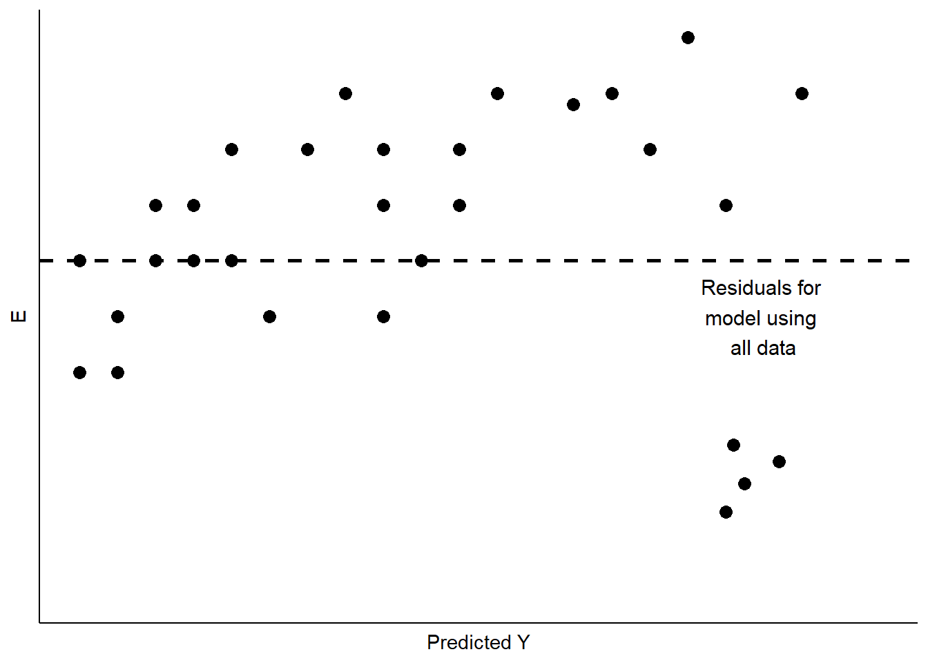
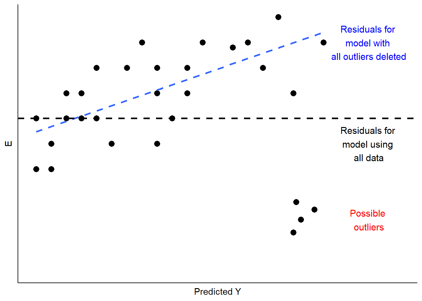
Figure \(\PageIndex{3}\): Unusual Data Patterns in Residuals

This is a case of influential outliers. The effect of such outliers can be significant, as the OLS estimates of AA and BB seek to minimize overall squared error. In the case of Figure \(\PageIndex{3}\), the effect would be to shift the estimate of BB to accommodate the unusual observations, as illustrated in Figure \(\PageIndex{4}\). One possible response would be to omit the unusual observations, as shown in Figure \(\PageIndex{4}\). Another would be to consider, theoretically and empirically, why these observations are unusual. Are they, perhaps, miscoded? Or are they codes representing missing values (e.g., “-99”)?

If they are not mis-codes, perhaps these outlier observations manifest a different kind of relationship between XX and YY, which might in turn, require a revised theory and model. We will address some modeling options to address this possibility when we explore multiple regression, in Part III of this book.

Figure \(\PageIndex{4}\): Implications of Unusual Data Patterns in Residuals

In sum, outlier analysis looks at residuals for patterns in which some observations deviate widely from others. If that deviation is influential, changing estimates of AA and BB as shown in Figure \(\PageIndex{4}\), then you must examine the observations to determine whether they are miscoded. If not, you can evaluate whether the cases are theoretically distinct, such that the influence of XX on YY is likely to be different than for other cases. If you conclude that this is so, you will need to respecify your model to account for these differences. We will discuss some options for doing that later in this chapter, and again in our discussion of multiple regression.

10.2.2 Non-Constant Variance

A second thing to look for in visual diagnostics of residuals is non-constant variance or heteroscedasticity. In this case, the variation in the residuals over the range of predicted values for YY should be roughly even. A problem occurs when that variation changes substantially as the predicted value of YY changes, as is illustrated in Figure \(\PageIndex{5}\).

##    x5           y5    z5
## 1   1  0.116268529 first
## 2   2 -0.058592447 first
## 3   3  0.178546500 first
## 4   4 -0.133259371 first
## 5   5 -0.044656677 first
## 6   6  0.056960612 first
## 7   7 -0.288971761 first
## 8   8 -0.086901834 first
## 9   9 -0.046170268 first
## 10 10 -0.055554091 first
## 11 11 -0.002013537 first
## 12 12 -0.015038222 first
## 13 13 -0.062812676 first
## 14 14  0.132322085 first
## 15 15 -0.152135057 first
## 16 16 -0.043742787 first
## 17 17  0.097057758 first
## 18 18  0.002822264 first
## 19 19 -0.008578219 first
## 20 20  0.038921440 first
## 21 21  0.023668737 first

##    x5          y5     z5
## 1  21  -0.7944212 second
## 2  22   3.9722634 second
## 3  23   2.0344877 second
## 4  24  -1.3313647 second
## 5  25  -8.0963483 second
## 6  26  -3.2788775 second
## 7  27  -6.3068507 second
## 8  28 -13.6105004 second
## 9  29  -3.3742972 second
## 10 30  -1.1897133 second
## 11 31   8.7458017 second
## 12 32   8.5587880 second
## 13 33   6.0964799 second
## 14 34  -6.0353801 second
## 15 35 -10.2333314 second
## 16 36  -5.0246837 second
## 17 37   6.8506290 second
## 18 38   0.4832010 second
## 19 39   2.3291504 second
## 20 40  -4.5016566 second
## 21 41  -8.4841231 second

##    x5            y5     z5
## 1   1   0.116268529  first
## 2   2  -0.058592447  first
## 3   3   0.178546500  first
## 4   4  -0.133259371  first
## 5   5  -0.044656677  first
## 6   6   0.056960612  first
## 7   7  -0.288971761  first
## 8   8  -0.086901834  first
## 9   9  -0.046170268  first
## 10 10  -0.055554091  first
## 11 11  -0.002013537  first
## 12 12  -0.015038222  first
## 13 13  -0.062812676  first
## 14 14   0.132322085  first
## 15 15  -0.152135057  first
## 16 16  -0.043742787  first
## 17 17   0.097057758  first
## 18 18   0.002822264  first
## 19 19  -0.008578219  first
## 20 20   0.038921440  first
## 21 21   0.023668737  first
## 22 21  -0.794421247 second
## 23 22   3.972263354 second
## 24 23   2.034487716 second
## 25 24  -1.331364730 second
## 26 25  -8.096348251 second
## 27 26  -3.278877502 second
## 28 27  -6.306850722 second
## 29 28 -13.610500382 second
## 30 29  -3.374297181 second
## 31 30  -1.189713327 second
## 32 31   8.745801727 second
## 33 32   8.558788016 second
## 34 33   6.096479914 second
## 35 34  -6.035380147 second
## 36 35 -10.233331440 second
## 37 36  -5.024683664 second
## 38 37   6.850629016 second
## 39 38   0.483200951 second
## 40 39   2.329150423 second
## 41 40  -4.501656591 second
## 42 41  -8.484123104 second

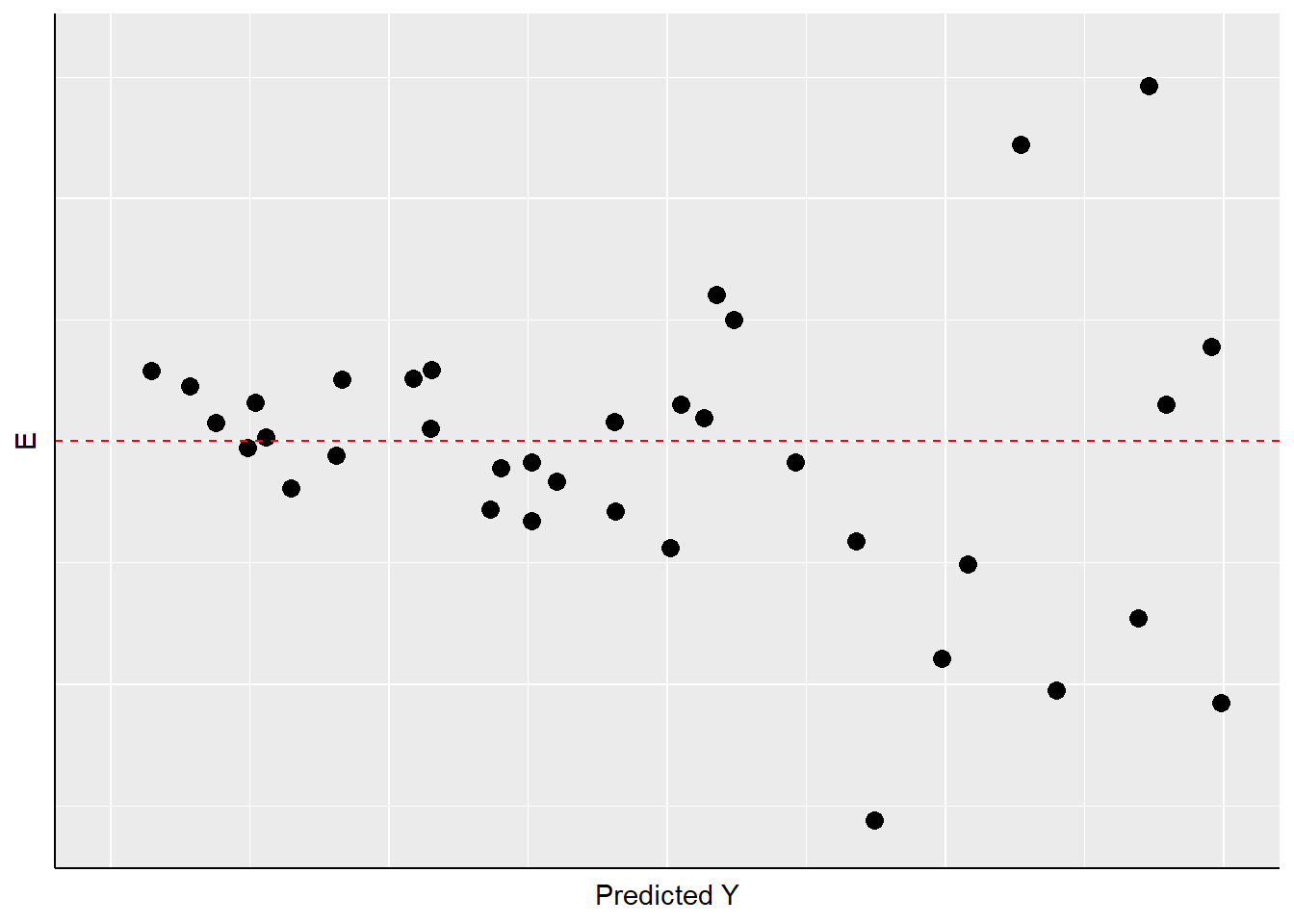
Figure \(\PageIndex{5}\): Non-Constant Variance in the Residuals

As Figure \(\PageIndex{5}\) shows, the width of the spread of the residuals grows as the predicted value of YY increases, making a fan-shaped pattern. Equally concerning would be a case of a “reverse fan”, or a pattern with a bulge in the middle and very “tight” distributions of residuals at either extreme. These would all be cases in which the assumption of constant-variance in the residuals (or “homoscedasticity”) fails, and are referred to as instances of heteroscedasticity.

What are the implications of heteroscedasticity? Our hypothesis tests for the estimated coefficients (AA and BB) are based on the assumption that the standard errors of the estimates (see the prior chapter) are normally distributed. If inspection of your residuals provides evidence to question that assumption, then the interpretation of the t-values and p-values may be problematic. Intuitively, in such a case the precision of our estimates of AA and BB are not constant – but rather will depend on the predicted value of YY. So you might be estimating BB relatively precisely in some ranges of YY, and less precise in others. That means you cannot depend on the estimated t and p-values to test your hypotheses.

10.2.3 Non-Linearity in the Parameters

One of the primary assumptions of simple OLS regression is that the estimated slope parameter (the BB) will be constant, and therefore the model will be linear. Put differently, the effect of any change in XX on YY should be constant over the range of YY. Thus, if our assumption is correct, the pattern of the residuals should be roughly symmetric, above and below zero, over the range of predicted values.

If the real relationship between XX and YY is not linear, however, the predicted (linear) values for YY will systematically depart from the (curved) relationship that is represented in the data. Figure \(\PageIndex{6}\) shows the kind of pattern we would expect in our residuals if the observed relationship between XX and YY is a strong curve when we attempt to model it as if it were linear.

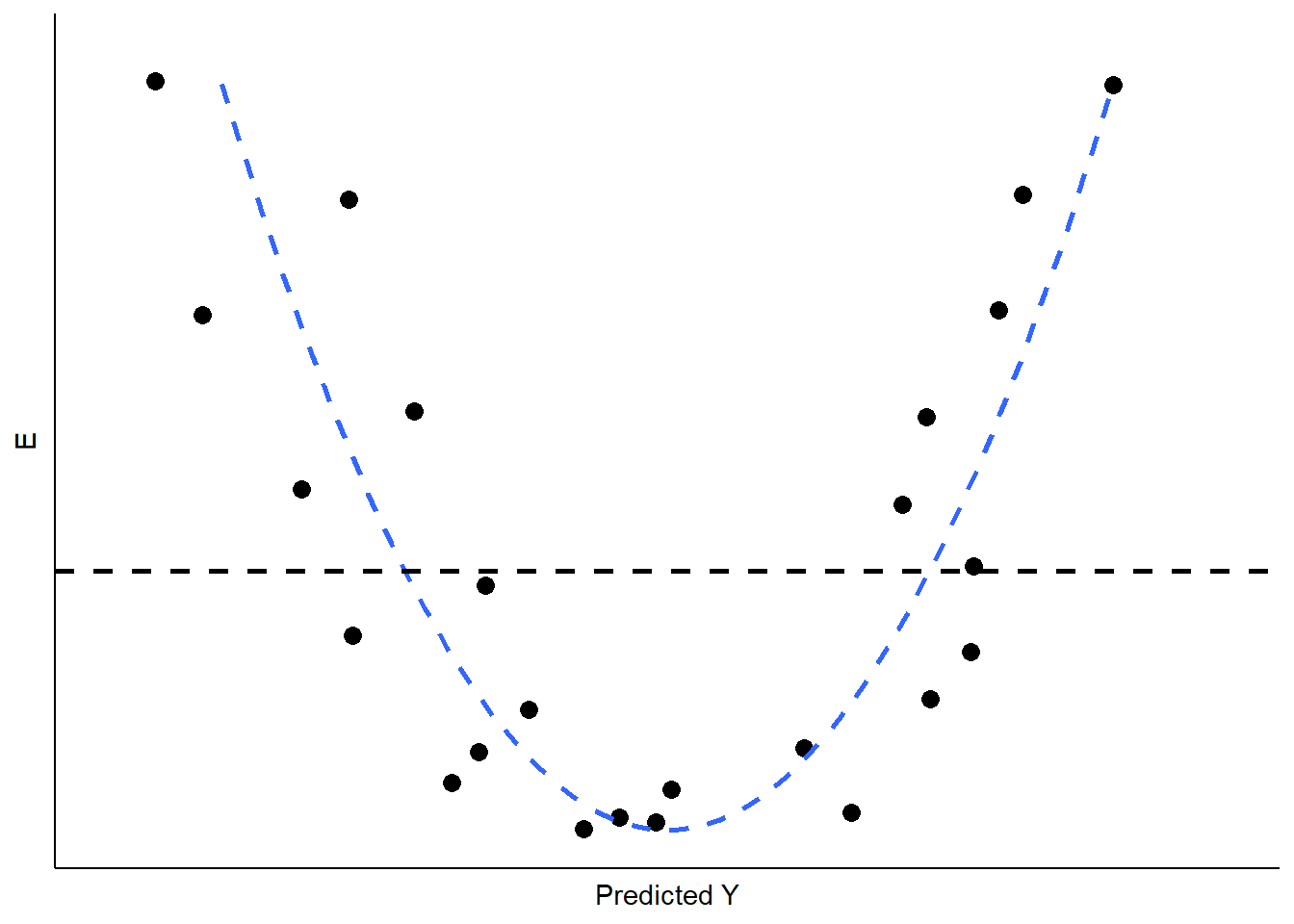
Figure \(\PageIndex{6}\): Non-Linearity in the Residuals

What are the implications of non-linearity? First, because the slope is non-constant, the estimate of BB will be biased. In the illustration shown in Figure \(\PageIndex{6}\), BB would underestimate the value of YY in both the low and high ranges of the predicted value of YY, and overestimate it in the mid-range. In addition, the standard errors of the residuals will be large, due to systematic over- and under-estimation of YY, making the model very inefficient (or imprecise).