5.3: Inferences to the Population from the Sample

Another key implication of the Central Limit Theorem that is illustrated in Figure \(\PageIndex{5}\) is that the mean of the repeated sample means is the same, regardless of sample size, and that the mean of the sample means is the population mean (assuming a large enough number of samples). Those conclusions lead to the important point that the sample mean is the best estimate of the population mean, i.e., the sample mean is an unbiased estimate of the population mean. Figure \(\PageIndex{5}\) also illustrates as the sample size increases, the efficiency of the estimate increases. As the sample size increases, the mean of any particular sample is more likely to approximate the population mean.

When we begin our research we should have some population in mind - the set of items that we want to draw conclusions about. We might want to know about all adult Americans or about human beings (past, present, and future) or about a specific meteorological condition. There is only one way to know with certainty about that population and that is to examine all cases that fit the definition of our population. Most of the time, though, we cannot do that – in the case of adult Americans it would be very time-consuming, expensive, and logistically quite challenging, and in the other two cases it simply would be impossible. Our research, then, often forces us to rely on samples.

Because we rely on samples, inferential statistics are probability-based. As Figure \(\PageIndex{5}\) illustrates, our sample could perfectly reflect our population; it could be (and is likely to be) at least a reasonable approximation of the population, or the sample could deviate substantially from the population. Two critical points are being made here: the best estimates we have of our population parameters are our sample statistics, and we never know with certainty how good that estimate is. We make decisions (statistical and real-world) based on probabilities.

5.3.1 Confidence Intervals

Because we are dealing with probabilities, if we are estimating a population parameter using a sample statistic, we will want to know how much confidence to place in that estimate. If we want to know a population mean, but only have a sample, the best estimate of that population mean is the sample mean. To know how much confidence to have in a sample mean, we put a confidence interval" around it. A confidence interval will report both a range for the estimate and the probability the population value falls in that range. We say, for example, that we are 95% confident that the true value is between A and B.

To find that confidence interval, we rely on the standard error of the estimate. Figure \(\PageIndex{5}\) plots the distribution of sample statistics drawn from repeated samples. As the sample size increases, the estimates cluster closer to the true population value, i.e., the standard deviation is smaller. We could use the standard deviation from repeated samples to determine the confidence we can have in any particular sample, but in reality, we are no more likely to draw repeated samples than we are to study the entire population. The standard error, though, provides an estimate of the standard deviation we would have if we did draw a number of samples. The standard error is based on the sample size and the distribution of observations in our data:

\[SE=s√n(5.3)(5.3)SE=sn\]

where ss is the sample standard deviation, and nn is the size (number of observations) of the sample.

The standard error can be interpreted just like a standard deviation. If we have a large sample, we can say that 68.26% of all of our samples (assuming we drew repeated samples) would fall within one standard error of our sample statistic or that 95.44% would fall within two standard errors.

If our sample size is not large, instead of using z-scores to estimate confidence intervals, we use t-scores to estimate the interval. T-scores are calculated just like z-score, but our interpretation of them is slightly different. The confidence interval formula is:

\[¯x+/−SEx∗t(5.4)(5.4)x¯+/−SEx∗t\]

To find the appropriate value for t, we need to decide what level of confidence we want (generally 95%) and our degrees of freedom (df), which is n−1n−1. We can find a confidence interval with R using the t.test function. By default, t.test will test the hypothesis that the mean of our variable of interest (glbcc_risk) is equal to zero. It will also find the mean score and a confidence interval for the glbcc_risk variable:

t.test(ds$glbcc_risk)

## 
##  One Sample t-test
## 
## data:  ds$glbcc_risk
## t = 97.495, df = 2535, p-value < 0.00000000000000022
## alternative hypothesis: true mean is not equal to 0
## 95 percent confidence interval:
##  5.826388 6.065568
## sample estimates:
## mean of x 
##  5.945978

Moving from the bottom up on the output we see that our mean score is 5.95. Next, we see that the 95% confidence interval is between 5.83 and 6.07. We are, therefore, 95% confident that the population mean is somewhere between those two scores. The first part of the output tests the null hypothesis that the mean value is equal to zero – a topic we will cover in the next section.

5.3.2 The Logic of Hypothesis Testing

We can use the same set of tools to test hypotheses. In this section, we introduce the logic of hypothesis testing. In the next chapter, we address it in more detail. Remember that a hypothesis is a statement about the way the world is and that it may be true or false. Hypotheses are generally deduced from our theory and if our expectations are confirmed, we gain confidence in our theory. Hypothesis testing is where our ideas meet the real world.

Due to the nature of inferential statistics, we cannot directly test hypotheses, but instead, we can test a null hypothesis. While a hypothesis is a statement of an expected relationship between two variables, the null hypothesis is a statement that says there is no relationship between the two variables. A null hypothesis might read: As XX increases, YY does not change. (We will discuss this topic more in the next chapter, but we want to understand the logic of the process here.)

Suppose a principal wants to cut down on absenteeism in her school and offers an incentive program for perfect attendance. Before the program, suppose the attendance rate was 85%. After having the new program in place for a while, she wants to know what the current rate is so she takes a sample of days and estimates the current attendance rate to be 88%. Her research hypothesis is: the attendance rate has gone up since the announcement of the new program (i.e., attendance is great than 85%). Her null hypothesis is that the attendance rate has not gone up since the announcement of the new program (i.e. attendance is less than or equal to 85%). At first, it seems that her null hypothesis is wrong (88%>85%)(88%>85%), but since we are using a sample, it is possible that the true population value is less than 85%. Based on her sample, how likely is it that the true population value is less than 85%? If the likelihood is small (and remember there will always be some chance), then we say our null hypothesis is wrong, i.e., we reject our null hypothesis, but if the likelihood is reasonable we accept our null hypothesis. The standard we normally use to make that determination is .05 – we want less than a .05 probability that we could have found our sample value (here 88%) if our null hypothesized value (85%) is true for the population. We use the t-statistic to find that probability. The formula is:

\[t=x−μse(5.5)(5.5)t=x−μse\]

If we return to the output presented above on glbcc_risk, we can see that R tested the null hypothesis that the true population value glbcc_risk is equal to zero. It reports t = 97.495 and a p-value of 2.2e-16. This p-value is less than .05, so we can reject our null hypothesis and be very confident that the true population value is greater than zero. % of the above items can be made dynamic.

5.3.3 Some Miscellaneous Notes about Hypothesis Testing

Before suspending our discussion of hypothesis testing, there are a few loose ends to tie up. First, you might be asking yourself where the .05 standard of hypothesis testing comes from. Is there some magic to that number? The answer is no“; .05 is simply the standard, but some researchers report .10 or .01. The p-value of .05, though, is generally considered to provide a reasonable balance between making it nearly impossible to reject a null hypothesis and too easily cluttering our knowledge box with things that we think are related but actually are not. Even using the .05 standard means that 5% of the time when we reject the null hypothesis, we are wrong - there is no relationship. (Besides giving you pause wondering what we are wrong about, it should also help you see why science deems replication to be so important.)

Second, as we just implied, anytime we make a decision to either accept or reject our null hypothesis, we could be wrong. The probabilities tell us that if p=0.05p=0.05, 5% of the time when we reject the null hypothesis, we are wrong because it is actually true. We call that type of mistake a Type I Error. However, when we accept the null hypothesis, we could also be wrong – there may be a relationship within the population. We call that a Type II Error. As should be evident, there is a trade-off between the two. If we decide to use a p-value of .01 instead of .05, we make fewer Type I errors – just one out of 100, instead of 5 out of 100. Yet that also means that we increase by .04 the likelihood that we are accepting a null hypothesis that is false – a Type II Error. To rephrase the previous paragraph: .05 is normally considered to be a reasonable balance between the probability of committing Type I Errors as opposed to Type II Errors. Of course, if the consequence of one type of error or the other is greater, then you can adjust the p-value.

Third, when testing hypotheses, we can use either a one-tailed test or a two-tailed test. The question is whether the entire .05 goes in one tailor is split evenly between the two tails (making, effectively, the p-value equal to .025). Generally speaking, if we have a directional hypothesis (e.g., as X increases so does Y), we will use a one-tail test. If we are expecting a positive relationship, but find a strong negative relationship, we generally conclude that we have a sampling quirk and that the relationship is null, rather than the opposite of what we expected. If, for some reason, you have a hypothesis that does not specify the direction, you would be interested in values in either tail and use a two-tailed test.

5.4 Differences Between Groups

In addition to covariance and correlation (discussed in the next chapter), we can also examine differences in some variables of interest between two or more groups. For example, we may want to compare the mean of the perceived climate change risk variable for males and females. First, we can examine these variables visually.

As coded in our dataset, gender (gender) is a numeric variable with a 1 for males and 0 for females. However, we may want to make gender a categorical variable with labels for Female and Male, as opposed to a numeric variable coded as 0’s and 1’s. To do this we make a new variable and use the factor command, which will tell R that the new variable is a categorical variable. Then we will tell R that this new variable has two levels or factors, Male and Female. Finally, we will label the factors of our new variable and name it f.gend.

ds$f.gend <- factor(ds$gender, levels = c(0, 1), labels = c("Female","Male"))

We can then observe differences in the distributions of perceived risk for males and females by creating density curves:

library(tidyverse)
ds %>%
  drop_na(f.gend) %>%
  ggplot(aes(glbcc_risk)) +
  geom_density() +
  facet_wrap(~ f.gend, scales = "fixed")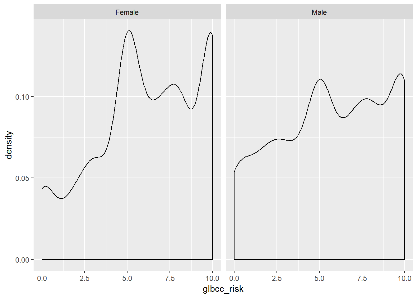

Figure \(\PageIndex{7}\): Density Plots of Climate Change Risk by Gender

Based on the density plots, it appears that some differences exist between males and females regarding perceived climate change risk. We can also use the by command to see the mean of climate change risk for males and females.

by(ds$glbcc_risk, ds$f.gend, mean, na.rm=TRUE)

## ds$f.gend: Female
## [1] 6.134259
## -------------------------------------------------------- 
## ds$f.gend: Male
## [1] 5.670577

Again there appears to be a difference, with females perceiving greater risk on average (6.13) than males (5.67). However, we want to know whether these differences are statistically significant. To test for the statistical significance of the difference between groups, we use a t-test.

5.4.1 t-tests

The t-test is based on the tt distribution. The tt distribution, also known as the Student’s tt distribution, is the probability distribution for sample estimates. It has similar properties and is related to, the normal distribution. The normal distribution is based on a population where μμ and σ2σ2 are known; however, the tt distribution is based on a sample where μμ and σ2σ2 are estimated, as the mean ¯XX¯ and variance s2xsx2. The mean of the tt distribution, like the normal distribution, is 00, but the variance, s2xsx2, is conditioned by n−1n−1 degrees of freedom(df). Degrees of freedom are the values used to calculate statistics that are “free” to vary.¹¹ A tt distribution approaches the standard normal distribution as the number of degrees of freedom increases.

In summary, we want to know the difference of means between males and females, d=¯Xm−¯Xfd=X¯m−X¯f, and if that difference is statistically significant. This amounts to a hypothesis test where our working hypothesis, H1H1, is that males are less likely than females to view climate change as risky. The null hypothesis, HAHA, is that there is no difference between males and females regarding the risks associated with climate change. To test H1H1 we use the t-test, which is calculated:

t=¯Xm−¯XfSEd(5.6)(5.6)t=X¯m−X¯fSEd

Where SEdSEd is the of the estimated differences between the two groups. To estimate SEdSEd, we need the SE of the estimated mean for each group. The SE is calculated:

SE=s√n(5.7)(5.7)SE=sn

where ss is the s.d. of the variable. H1H1 states that there is a difference between males and females, therefore under H1H1 it is expected that t>0t>0 since zero is the mean of the tt distribution. However, under HAHA it is expected that t=0t=0.

We can calculate this in R. First, we calculate the nn size for males and females. Then we calculate the SE for males and females.

n.total <- length(ds$gender)
nM <- sum(ds$gender, na.rm=TRUE)
nF <- n.total-nM
by(ds$glbcc_risk, ds$f.gend, sd, na.rm=TRUE)

## ds$f.gend: Female
## [1] 2.981938
## -------------------------------------------------------- 
## ds$f.gend: Male
## [1] 3.180171

sdM <- 2.82
seM <- 2.82/(sqrt(nM))
seM

## [1] 0.08803907

sdF <- 2.35
seF <- 2.35/(sqrt(nF))
seF

## [1] 0.06025641

Next, we need to calculate the SEdSEd:SEd=√SE2M+SE2F(5.8)(5.8)SEd=SEM2+SEF2

seD <- sqrt(seM^2+seF^2)
seD

## [1] 0.1066851

Finally, we can calculate our tt-score, and use the t.test function to check.

by(ds$glbcc_risk, ds$f.gend, mean, na.rm=TRUE)

## ds$f.gend: Female
## [1] 6.134259
## -------------------------------------------------------- 
## ds$f.gend: Male
## [1] 5.670577

meanF <- 6.96 
meanM <- 6.42
t <- (meanF-meanM)/seD
t

## [1] 5.061625

t.test(ds$glbcc_risk~ds$gender)

## 
##  Welch Two Sample t-test
## 
## data:  ds$glbcc_risk by ds$gender
## t = 3.6927, df = 2097.5, p-value = 0.0002275
## alternative hypothesis: true difference in means is not equal to 0
## 95 percent confidence interval:
##  0.2174340 0.7099311
## sample estimates:
## mean in group 0 mean in group 1 
##        6.134259        5.670577

For the difference in the perceived risk between women and men, we have a tt-value of 4.6. This result is greater than zero, as expected by H1H1. In addition, as shown in the t.test output the pp-value—the probability of obtaining our result if the population difference was 00—is extremely low at .0002275 (that’s the same as 2.275e-04). Therefore, we reject the null hypothesis and concluded that there are differences (on average) in the ways that males and females perceive climate change risk.

5.5 Summary

In this chapter we gained an understanding of inferential statistics, how to use them to place confidence intervals around an estimate, and an overview of how to use them to test hypotheses. In the next chapter, we turn, more formally, to testing hypotheses using crosstabs and by comparing means of different groups. We then continue to explore hypothesis testing and model building using regression analysis.

---

8. It is important to keep in mind that, for purposes of theory building, the population of interest may not be finite. For example, if you theorize about general properties of human behavior, many of the members of the human population are not yet (or are no longer) alive. Hence it is not possible to include all of the population of interest in your research. We therefore rely on samples.↩
9. Of course, we also need to estimate changes – both gradual and abrupt – in how people behave over time, which is the province of time-series analysis.↩
10. Wei Wang, David Rothschild, Sharad Goel, and Andrew Gelman (2014) ’’Forecasting Elections with Non-Representative Polls," Preprint submitted to International Journal of Forecasting March 31, 2014.↩
11. In a difference of means test across two groups, we “use up” one observation when we separate the observations into two groups. Hence the denominator reflects the loss of that used up observation: n-1.↩