15.2: Estimating a Linear Regression Model

Last updated
Save as PDF

Page ID: 4036

\( \newcommand{\vecs}[1]{\overset { \scriptstyle \rightharpoonup} {\mathbf{#1}} } \) \( \newcommand{\vecd}[1]{\overset{-\!-\!\rightharpoonup}{\vphantom{a}\smash {#1}}} \)\(\newcommand{\id}{\mathrm{id}}\) \( \newcommand{\Span}{\mathrm{span}}\) \( \newcommand{\kernel}{\mathrm{null}\,}\) \( \newcommand{\range}{\mathrm{range}\,}\) \( \newcommand{\RealPart}{\mathrm{Re}}\) \( \newcommand{\ImaginaryPart}{\mathrm{Im}}\) \( \newcommand{\Argument}{\mathrm{Arg}}\) \( \newcommand{\norm}[1]{\| #1 \|}\) \( \newcommand{\inner}[2]{\langle #1, #2 \rangle}\) \( \newcommand{\Span}{\mathrm{span}}\) \(\newcommand{\id}{\mathrm{id}}\) \( \newcommand{\Span}{\mathrm{span}}\) \( \newcommand{\kernel}{\mathrm{null}\,}\) \( \newcommand{\range}{\mathrm{range}\,}\) \( \newcommand{\RealPart}{\mathrm{Re}}\) \( \newcommand{\ImaginaryPart}{\mathrm{Im}}\) \( \newcommand{\Argument}{\mathrm{Arg}}\) \( \newcommand{\norm}[1]{\| #1 \|}\) \( \newcommand{\inner}[2]{\langle #1, #2 \rangle}\) \( \newcommand{\Span}{\mathrm{span}}\)\(\newcommand{\AA}{\unicode[.8,0]{x212B}}\)

Figure 15.4: A depiction of the residuals associated with the best fitting regression line

Figure 15.5: The residuals associated with a poor regression line

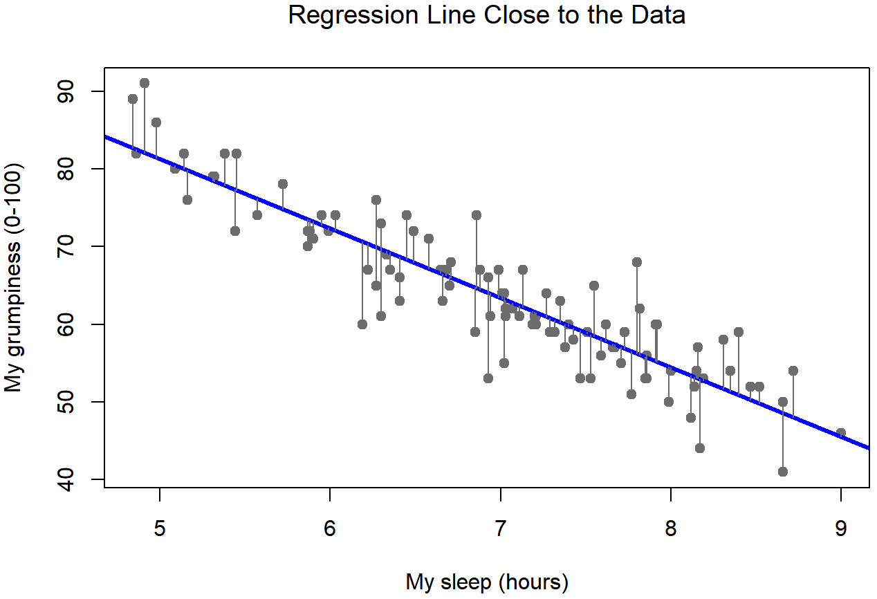
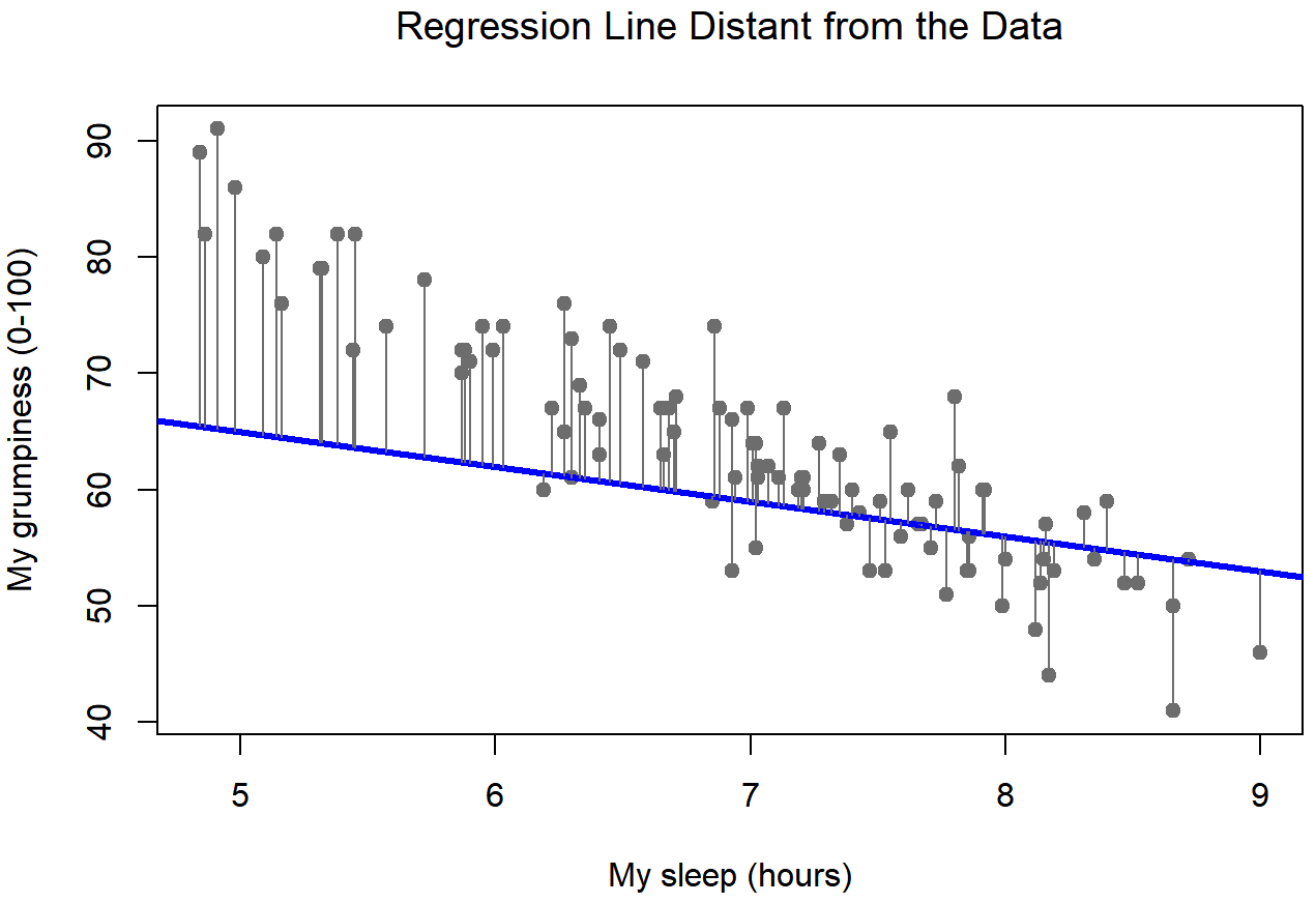
Okay, now let’s redraw our pictures, but this time I’ll add some lines to show the size of the residual for all observations. When the regression line is good, our residuals (the lengths of the solid black lines) all look pretty small, as shown in Figure 15.4, but when the regression line is a bad one, the residuals are a lot larger, as you can see from looking at Figure 15.5. Hm. Maybe what we “want” in a regression model is small residuals. Yes, that does seem to make sense. In fact, I think I’ll go so far as to say that the “best fitting” regression line is the one that has the smallest residuals. Or, better yet, since statisticians seem to like to take squares of everything why not say that …

The estimated regression coefficients, \(\ \hat{b_0}\) and \(\hat{b_1}\) are those that minimise the sum of the squared residuals, which we could either write as \(\sum_{i}\left(Y_{i}-\hat{Y}_{i}\right)^{2}\) or as \(\sum_{i} \epsilon_{i}^{2}\).

Yes, yes that sounds even better. And since I’ve indented it like that, it probably means that this is the right answer. And since this is the right answer, it’s probably worth making a note of the fact that our regression coefficients are estimates (we’re trying to guess the parameters that describe a population!), which is why I’ve added the little hats, so that we get \(\ \hat{b_0}\) and \(\ \hat{b_1}\) rather than b0 and b1. Finally, I should also note that – since there’s actually more than one way to estimate a regression model – the more technical name for this estimation process is ordinary least squares (OLS) regression.

At this point, we now have a concrete definition for what counts as our “best” choice of regression coefficients, \(\ \hat{b_0}\) and \(\ \hat{b_1}\). The natural question to ask next is, if our optimal regression coefficients are those that minimise the sum squared residuals, how do we find these wonderful numbers? The actual answer to this question is complicated, and it doesn’t help you understand the logic of regression.²¹⁵ As a result, this time I’m going to let you off the hook. Instead of showing you how to do it the long and tedious way first, and then “revealing” the wonderful shortcut that R provides you with, let’s cut straight to the chase… and use the lm() function (short for “linear model”) to do all the heavy lifting.

Using the `lm()` function

The lm() function is a fairly complicated one: if you type ?lm, the help files will reveal that there are a lot of arguments that you can specify, and most of them won’t make a lot of sense to you. At this stage however, there’s really only two of them that you care about, and as it turns out you’ve seen them before:

formula. A formula that specifies the regression model. For the simple linear regression models that we’ve talked about so far, in which you have a single predictor variable as well as an intercept term, this formula is of the form outcome ~ predictor. However, more complicated formulas are allowed, and we’ll discuss them later.
data. The data frame containing the variables.

As we saw with aov() in Chapter 14, the output of the lm() function is a fairly complicated object, with quite a lot of technical information buried under the hood. Because this technical information is used by other functions, it’s generally a good idea to create a variable that stores the results of your regression. With this in mind, to run my linear regression, the command I want to use is this:

regression.1 <- lm( formula = dan.grump ~ dan.sleep,  
                    data = parenthood )

Note that I used dan.grump ~ dan.sleep as the formula: in the model that I’m trying to estimate, dan.grump is the outcome variable, and dan.sleep is the predictor variable. It’s always a good idea to remember which one is which! Anyway, what this does is create an “lm object” (i.e., a variable whose class is "lm") called regression.1. Let’s have a look at what happens when we print() it out:

print( regression.1 )

## 
## Call:
## lm(formula = dan.grump ~ dan.sleep, data = parenthood)
## 
## Coefficients:
## (Intercept)    dan.sleep  
##     125.956       -8.937

This looks promising. There’s two separate pieces of information here. Firstly, R is politely reminding us what the command was that we used to specify the model in the first place, which can be helpful. More importantly from our perspective, however, is the second part, in which R gives us the intercept \(\ \hat{b_0}\) =125.96 and the slope \(\ \hat{b_1}\) =−8.94. In other words, the best-fitting regression line that I plotted in Figure 15.2 has this formula:

\(\ \hat{Y_i} = -8.94 \ X_i + 125.96\)

Interpreting the estimated model

The most important thing to be able to understand is how to interpret these coefficients. Let’s start with \(\ \hat{b_1}\), the slope. If we remember the definition of the slope, a regression coefficient of \(\ \hat{b_1}\) =−8.94 means that if I increase X_i by 1, then I’m decreasing Y_i by 8.94. That is, each additional hour of sleep that I gain will improve my mood, reducing my grumpiness by 8.94 grumpiness points. What about the intercept? Well, since \(\ \hat{b_0}\) corresponds to “the expected value of Y_i when Xi equals 0”, it’s pretty straightforward. It implies that if I get zero hours of sleep (X_i=0) then my grumpiness will go off the scale, to an insane value of (Y_i=125.96). Best to be avoided, I think.