14.3: How ANOVA Works

In order to answer the question posed by our clinical trial data, we’re going to run a one-way ANOVA. As usual, I’m going to start by showing you how to do it the hard way, building the statistical tool from the ground up and showing you how you could do it in R if you didn’t have access to any of the cool built-in ANOVA functions. And, as always, I hope you’ll read it carefully, try to do it the long way once or twice to make sure you really understand how ANOVA works, and then – once you’ve grasped the concept – never ever do it this way again.

The experimental design that I described in the previous section strongly suggests that we’re interested in comparing the average mood change for the three different drugs. In that sense, we’re talking about an analysis similar to the t-test (Chapter 13, but involving more than two groups. If we let μ_P denote the population mean for the mood change induced by the placebo, and let μ_A and μ_J denote the corresponding means for our two drugs, Anxifree and Joyzepam, then the (somewhat pessimistic) null hypothesis that we want to test is that all three population means are identical: that is, neither of the two drugs is any more effective than a placebo. Mathematically, we write this null hypothesis like this:

H₀: it is true that μ_P=μ_A=μ_J

As a consequence, our alternative hypothesis is that at least one of the three different treatments is different from the others. It’s a little trickier to write this mathematically, because (as we’ll discuss) there are quite a few different ways in which the null hypothesis can be false. So for now we’ll just write the alternative hypothesis like this:

H₁: it is *not* true that μ_P=μ_A=μ_J

This null hypothesis is a lot trickier to test than any of the ones we’ve seen previously. How shall we do it? A sensible guess would be to “do an ANOVA”, since that’s the title of the chapter, but it’s not particularly clear why an “analysis of variances” will help us learn anything useful about the means. In fact, this is one of the biggest conceptual difficulties that people have when first encountering ANOVA. To see how this works, I find it most helpful to start by talking about variances. In fact, what I’m going to do is start by playing some mathematical games with the formula that describes the variance. That is, we’ll start out by playing around with variances, and it will turn out that this gives us a useful tool for investigating means.

formulas for the variance of Y

Firstly, let’s start by introducing some notation. We’ll use G to refer to the total number of groups. For our data set, there are three drugs, so there are G=3 groups. Next, we’ll use N to refer to the total sample size: there are a total of N=18 people in our data set. Similarly, let’s use N_k to denote the number of people in the k-th group. In our fake clinical trial, the sample size is N_k=6 for all three groups.²⁰¹ Finally, we’ll use Y to denote the outcome variable: in our case, Y refers to mood change. Specifically, we’ll use Y_ik to refer to the mood change experienced by the i-th member of the k-th group. Similarly, we’ll use \(\ \bar{Y}\) to be the average mood change, taken across all 18 people in the experiment, and \(\ \bar{Y_k}\) to refer to the average mood change experienced by the 6 people in group k.

Excellent. Now that we’ve got our notation sorted out, we can start writing down formulas. To start with, let’s recall the formula for the variance that we used in Section 5.2, way back in those kinder days when we were just doing descriptive statistics. The sample variance of Y is defined as follows:

\(\operatorname{Var}(Y)=\dfrac{1}{N} \sum_{k=1}^{G} \sum_{i=1}^{N_{k}}\left(Y_{i k}-\bar{Y}\right)^{2}\)

This formula looks pretty much identical to the formula for the variance in Section 5.2. The only difference is that this time around I’ve got two summations here: I’m summing over groups (i.e., values for k) and over the people within the groups (i.e., values for i). This is purely a cosmetic detail: if I’d instead used the notation Y_p to refer to the value of the outcome variable for person p in the sample, then I’d only have a single summation. The only reason that we have a double summation here is that I’ve classified people into groups, and then assigned numbers to people within groups.

A concrete example might be useful here. Let’s consider this table, in which we have a total of N=5 people sorted into G=2 groups. Arbitrarily, let’s say that the “cool” people are group 1, and the “uncool” people are group 2, and it turns out that we have three cool people (N₁=3) and two uncool people (N₂=2).

name	person (p)	group	group num (k)	index in group (i)	grumpiness (Yik or Yp)
Ann	1	cool	1	1	20
Ben	2	cool	1	2	55
Cat	3	cool	1	3	21
Dan	4	uncool	2	1	91
Egg	5	uncool	2	2	22

Notice that I’ve constructed two different labelling schemes here. We have a “person” variable p, so it would be perfectly sensible to refer to Y_p as the grumpiness of the p-th person in the sample. For instance, the table shows that Dan is the four so we’d say p=4. So, when talking about the grumpiness Y of this “Dan” person, whoever he might be, we could refer to his grumpiness by saying that Y_p=91, for person p=4 that is. However, that’s not the only way we could refer to Dan. As an alternative we could note that Dan belongs to the “uncool” group (k=2), and is in fact the first person listed in the uncool group (i=1). So it’s equally valid to refer to Dan’s grumpiness by saying that Y_ik=91, where k=2 and i=1. In other words, each person p corresponds to a unique ik combination, and so the formula that I gave above is actually identical to our original formula for the variance, which would be

\(\operatorname{Var}(Y)=\dfrac{1}{N} \sum_{p=1}^{N}\left(Y_{p}-\bar{Y}\right)^{2}\)

In both formulas, all we’re doing is summing over all of the observations in the sample. Most of the time we would just use the simpler Y_p notation: the equation using Y_p is clearly the simpler of the two. However, when doing an ANOVA it’s important to keep track of which participants belong in which groups, and we need to use the Y_ik notation to do this.

From variances to sums of squares

Okay, now that we’ve got a good grasp on how the variance is calculated, let’s define something called the total sum of squares, which is denoted SS_tot. This is very simple: instead of averaging the squared deviations, which is what we do when calculating the variance, we just add them up. So the formula for the total sum of squares is almost identical to the formula for the variance:

\(\mathrm{SS}_{t o t}=\sum_{k=1}^{G} \sum_{i=1}^{N_{k}}\left(Y_{i k}-\bar{Y}\right)^{2}\)

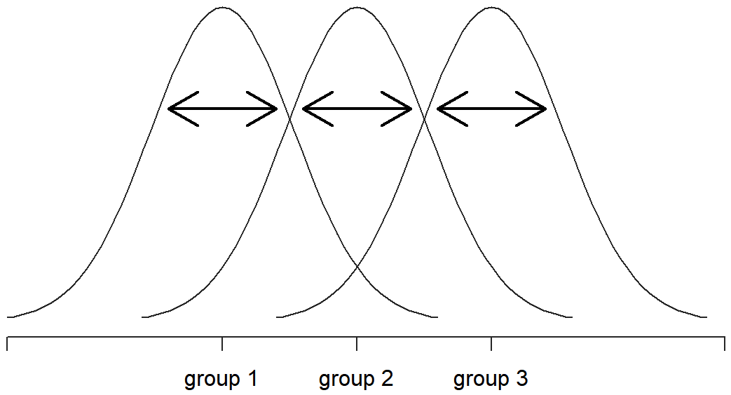
When we talk about analysing variances in the context of ANOVA, what we’re really doing is working with the total sums of squares rather than the actual variance. One very nice thing about the total sum of squares is that we can break it up into two different kinds of variation. Firstly, we can talk about the within-group sum of squares, in which we look to see how different each individual person is from their own group mean:

\(\mathrm{SS}_{w}=\sum_{k=1}^{G} \sum_{i=1}^{N_{k}}\left(Y_{i k}-\bar{Y}_{k}\right)^{2}\)

where \(\ \bar{Y_k}\) is a group mean. In our example, \(\ \bar{Y_k}\) would be the average mood change experienced by those people given the k-th drug. So, instead of comparing individuals to the average of all people in the experiment, we’re only comparing them to those people in the the same group. As a consequence, you’d expect the value of SS_w to be smaller than the total sum of squares, because it’s completely ignoring any group differences – that is, the fact that the drugs (if they work) will have different effects on people’s moods.

Next, we can define a third notion of variation which captures only the differences between groups. We do this by looking at the differences between the group means \(\ \bar{Y_k}\) and grand mean \(\ \bar{Y}\). In order to quantify the extent of this variation, what we do is calculate the between-group sum of squares:

\(\begin{aligned} \mathrm{SS}_{b} &=\sum_{k=1}^{G} \sum_{i=1}^{N_{k}}\left(\bar{Y}_{k}-\bar{Y}\right)^{2} \\ &=\sum_{k=1}^{G} N_{k}\left(\bar{Y}_{k}-\bar{Y}\right)^{2} \end{aligned}\)

It’s not too difficult to show that the total variation among people in the experiment SS_tot is actually the sum of the differences between the groups SS_b and the variation inside the groups SS_w. That is:

SS_w+SS_b=SS_tot

Yay.

Figure 14.2: Graphical illustration of “between groups” variation

Figure 14.3: Graphical illustration of “within groups” variation

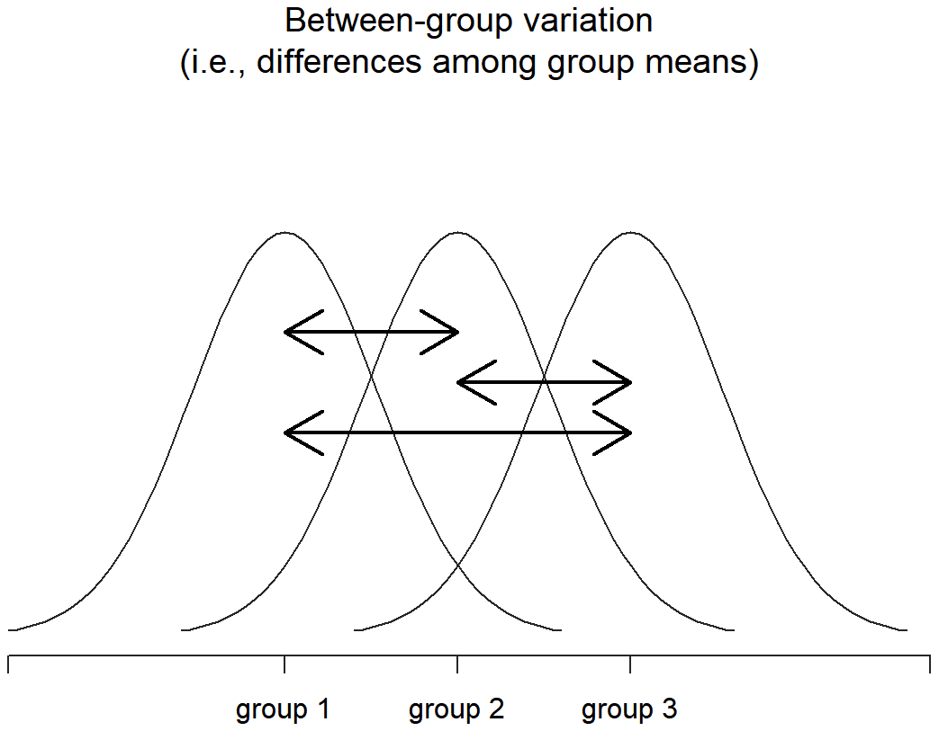
Okay, so what have we found out? We’ve discovered that the total variability associated with the outcome variable (SS_tot) can be mathematically carved up into the sum of “the variation due to the differences in the sample means for the different groups” (SS_b) plus “all the rest of the variation” (SS_w). How does that help me find out whether the groups have different population means? Um. Wait. Hold on a second… now that I think about it, this is exactly what we were looking for. If the null hypothesis is true, then you’d expect all the sample means to be pretty similar to each other, right? And that would imply that you’d expect SS_b to be really small, or at least you’d expect it to be a lot smaller than the “the variation associated with everything else”, SS_w. Hm. I detect a hypothesis test coming on…

From sums of squares to the F-test

As we saw in the last section, the qualitative idea behind ANOVA is to compare the two sums of squares values SS_b and SS_w to each other: if the between-group variation is SS_b is large relative to the within-group variation SS_w then we have reason to suspect that the population means for the different groups aren’t identical to each other. In order to convert this into a workable hypothesis test, there’s a little bit of “fiddling around” needed. What I’ll do is first show you what we do to calculate our test statistic – which is called an F ratio – and then try to give you a feel for why we do it this way.

In order to convert our SS values into an F-ratio, the first thing we need to calculate is the degrees of freedom associated with the SSb and SS_w values. As usual, the degrees of freedom corresponds to the number of unique “data points” that contribute to a particular calculation, minus the number of “constraints” that they need to satisfy. For the within-groups variability, what we’re calculating is the variation of the individual observations (N data points) around the group means (G constraints). In contrast, for the between groups variability, we’re interested in the variation of the group means (G data points) around the grand mean (1 constraint). Therefore, the degrees of freedom here are:

df_b=G−1

df_w=N−G

Okay, that seems simple enough. What we do next is convert our summed squares value into a “mean squares” value, which we do by dividing by the degrees of freedom:

\(\ MS_b = {SS_b \over df_b} \)

\(\ MS_w = {SS_w \over df_w} \)

Finally, we calculate the F-ratio by dividing the between-groups MS by the within-groups MS:

\(\ F={MS_b \over MS_w} \)

At a very general level, the intuition behind the F statistic is straightforward: bigger values of F means that the between-groups variation is large, relative to the within-groups variation. As a consequence, the larger the value of F, the more evidence we have against the null hypothesis. But how large does F have to be in order to actually reject H₀? In order to understand this, you need a slightly deeper understanding of what ANOVA is and what the mean squares values actually are.

The next section discusses that in a bit of detail, but for readers that aren’t interested in the details of what the test is actually measuring, I’ll cut to the chase. In order to complete our hypothesis test, we need to know the sampling distribution for F if the null hypothesis is true. Not surprisingly, the sampling distribution for the F statistic under the null hypothesis is an F distribution. If you recall back to our discussion of the F distribution in Chapter @ref(probability, the F distribution has two parameters, corresponding to the two degrees of freedom involved: the first one df1 is the between groups degrees of freedom dfb, and the second one df2 is the within groups degrees of freedom df_w.

A summary of all the key quantities involved in a one-way ANOVA, including the formulas showing how they are calculated, is shown in Table 14.1.

Table 14.1: All of the key quantities involved in an ANOVA, organised into a “standard” ANOVA table. The formulas for all quantities (except the p-value, which has a very ugly formula and would be nightmarishly hard to calculate without a computer) are shown.

	df	sum of squares	mean squares	F statistic	p value
between groups	dfb=G−1	\(\mathrm{SS}_{b}=\sum_{k=1}^{G} N_{k}\left(\bar{Y}_{k}-\bar{Y}\right)^{2}\)	\(\mathrm{MS}_{b}=\dfrac{\mathrm{SS}_{b}}{\mathrm{df}_{b}}\)	\(F=\dfrac{\mathrm{MS}_{b}}{\mathrm{MS}_{w}}\)	[complicated]
within groups	dfw=N−G	\(SS_w=\sum_{k=1}^{G} \sum_{i=1}^{N_{k}}\left(Y_{i k}-\bar{Y}_{k}\right)^{2}\)	\(\mathrm{MS}_{w}=\dfrac{\mathrm{SS}_{w}}{\mathrm{df}_{w}}\)	-	-

model for the data and the meaning of F (advanced)

At a fundamental level, ANOVA is a competition between two different statistical models, H₀ and H₁. When I described the null and alternative hypotheses at the start of the section, I was a little imprecise about what these models actually are. I’ll remedy that now, though you probably won’t like me for doing so. If you recall, our null hypothesis was that all of the group means are identical to one another. If so, then a natural way to think about the outcome variable Y_ik is to describe individual scores in terms of a single population mean μ, plus the deviation from that population mean. This deviation is usually denoted ϵ_ik and is traditionally called the error or residual associated with that observation. Be careful though: just like we saw with the word “significant”, the word “error” has a technical meaning in statistics that isn’t quite the same as its everyday English definition. In everyday language, “error” implies a mistake of some kind; in statistics, it doesn’t (or at least, not necessarily). With that in mind, the word “residual” is a better term than the word “error”. In statistics, both words mean “leftover variability”: that is, “stuff” that the model can’t explain. In any case, here’s what the null hypothesis looks like when we write it as a statistical model:

Y_ik=μ+ϵ_ik

where we make the assumption (discussed later) that the residual values ϵ_ik are normally distributed, with mean 0 and a standard deviation σ that is the same for all groups. To use the notation that we introduced in Chapter 9 we would write this assumption like this:

ϵ_ik∼Normal(0,σ²)

What about the alternative hypothesis, H₁? The only difference between the null hypothesis and the alternative hypothesis is that we allow each group to have a different population mean. So, if we let μk denote the population mean for the k-th group in our experiment, then the statistical model corresponding to H₁ is:

Y_ik=μ_k+ϵ_ik

where, once again, we assume that the error terms are normally distributed with mean 0 and standard deviation σ. That is, the alternative hypothesis also assumes that

ϵ∼Normal(0,σ²)

Okay, now that we’ve described the statistical models underpinning H₀ and H₁ in more detail, it’s now pretty straightforward to say what the mean square values are measuring, and what this means for the interpretation of F. I won’t bore you with the proof of this, but it turns out that the within-groups mean square, MS_w, can be viewed as an estimator (in the technical sense: Chapter 10 of the error variance σ². The between-groups mean square MS_b is also an estimator; but what it estimates is the error variance plus a quantity that depends on the true differences among the group means. If we call this quantity Q, then we can see that the F-statistic is basically²⁰²

\(F=\dfrac{\hat{Q}+\hat{\sigma}^{2}}{\hat{\sigma}^{2}}\)

where the true value Q=0 if the null hypothesis is true, and Q>0 if the alternative hypothesis is true (e.g. ch. 10 Hays 1994). Therefore, at a bare minimum the F value must be larger than 1 to have any chance of rejecting the null hypothesis. Note that this doesn’t mean that it’s impossible to get an F-value less than 1. What it means is that, if the null hypothesis is true the sampling distribution of the F ratio has a mean of 1,²⁰³ and so we need to see F-values larger than 1 in order to safely reject the null.

To be a bit more precise about the sampling distribution, notice that if the null hypothesis is true, both MS_b and MS_w are estimators of the variance of the residuals ϵ_ik. If those residuals are normally distributed, then you might suspect that the estimate of the variance of ϵ_ik is chi-square distributed… because (as discussed in Section 9.6 that’s what a chi-square distribution is: it’s what you get when you square a bunch of normally-distributed things and add them up. And since the F distribution is (again, by definition) what you get when you take the ratio between two things that are X² distributed… we have our sampling distribution. Obviously, I’m glossing over a whole lot of stuff when I say this, but in broad terms, this really is where our sampling distribution comes from.

worked example

The previous discussion was fairly abstract, and a little on the technical side, so I think that at this point it might be useful to see a worked example. For that, let’s go back to the clinical trial data that I introduced at the start of the chapter. The descriptive statistics that we calculated at the beginning tell us our group means: an average mood gain of 0.45 for the placebo, 0.72 for Anxifree, and 1.48 for Joyzepam. With that in mind, let’s party like it’s 1899²⁰⁴ and start doing some pencil and paper calculations. I’ll only do this for the first 5 observations, because it’s not bloody 1899 and I’m very lazy. Let’s start by calculating SS_w, the within-group sums of squares. First, let’s draw up a nice table to help us with our calculations…

group (k)	outcome (Yik)
placebo	0.5
placebo	0.3
placebo	0.1
anxifree	0.6
anxifree	0.4

At this stage, the only thing I’ve included in the table is the raw data itself: that is, the grouping variable (i.e., drug) and outcome variable (i.e. mood.gain) for each person. Note that the outcome variable here corresponds to the Y_ik value in our equation previously. The next step in the calculation is to write down, for each person in the study, the corresponding group mean; that is, \(\ \bar{Y_k}\). This is slightly repetitive, but not particularly difficult since we already calculated those group means when doing our descriptive statistics:

group (k)	outcome (Yik)	group mean (\(\ \bar{Y_k}\)
placebo	0.5	0.45
placebo	0.3	0.45
placebo	0.1	0.45
anxifree	0.6	0.72
anxifree	0.4	0.72

Now that we’ve written those down, we need to calculate – again for every person – the deviation from the corresponding group mean. That is, we want to subtract Y_ik−\(\ \bar{Y_k}\). After we’ve done that, we need to square everything. When we do that, here’s what we get:

group (k)	outcome (Yik)	group mean (\(\ \bar{Y_k}\))	dev. from group mean (Yik−\(\ \bar{Y_k}\))	squared deviation ((Yik−\(\ \bar{Y_k}\))^2)
placebo	0.5	0.45	0.05	0.0025
placebo	0.3	0.45	-0.15	0.0225
placebo	0.1	0.45	-0.35	0.1225
anxifree	0.6	0.72	-0.12	0.0136
anxifree	0.4	0.72	-0.32	0.1003

The last step is equally straightforward. In order to calculate the within-group sum of squares, we just add up the squared deviations across all observations:

\(\begin{aligned} \mathrm{SS}_{w} &=0.0025+0.0225+0.1225+0.0136+0.1003 \\ &=0.2614 \end{aligned}\)

Of course, if we actually wanted to get the right answer, we’d need to do this for all 18 observations in the data set, not just the first five. We could continue with the pencil and paper calculations if we wanted to, but it’s pretty tedious. Alternatively, it’s not too hard to get R to do it. Here’s how:

outcome <- clin.trial$mood.gain
group <- clin.trial$drug
gp.means <- tapply(outcome,group,mean)
gp.means <- gp.means[group]
dev.from.gp.means <- outcome - gp.means
squared.devs <- dev.from.gp.means ^2

It might not be obvious from inspection what these commands are doing: as a general rule, the human brain seems to just shut down when faced with a big block of programming. However, I strongly suggest that – if you’re like me and tend to find that the mere sight of this code makes you want to look away and see if there’s any beer left in the fridge or a game of footy on the telly – you take a moment and look closely at these commands one at a time. Every single one of these commands is something you’ve seen before somewhere else in the book. There’s nothing novel about them (though I’ll have to admit that the tapply() function takes a while to get a handle on), so if you’re not quite sure how these commands work, this might be a good time to try playing around with them yourself, to try to get a sense of what’s happening. On the other hand, if this does seem to make sense, then you won’t be all that surprised at what happens when I wrap these variables in a data frame, and print it out…

Y <- data.frame( group, outcome, gp.means,
                  dev.from.gp.means, squared.devs )
print(Y, digits = 2)

##       group outcome gp.means dev.from.gp.means squared.devs
## 1   placebo     0.5     0.45             0.050       0.0025
## 2   placebo     0.3     0.45            -0.150       0.0225
## 3   placebo     0.1     0.45            -0.350       0.1225
## 4  anxifree     0.6     0.72            -0.117       0.0136
## 5  anxifree     0.4     0.72            -0.317       0.1003
## 6  anxifree     0.2     0.72            -0.517       0.2669
## 7  joyzepam     1.4     1.48            -0.083       0.0069
## 8  joyzepam     1.7     1.48             0.217       0.0469
## 9  joyzepam     1.3     1.48            -0.183       0.0336
## 10  placebo     0.6     0.45             0.150       0.0225
## 11  placebo     0.9     0.45             0.450       0.2025
## 12  placebo     0.3     0.45            -0.150       0.0225
## 13 anxifree     1.1     0.72             0.383       0.1469
## 14 anxifree     0.8     0.72             0.083       0.0069
## 15 anxifree     1.2     0.72             0.483       0.2336
## 16 joyzepam     1.8     1.48             0.317       0.1003
## 17 joyzepam     1.3     1.48            -0.183       0.0336
## 18 joyzepam     1.4     1.48            -0.083       0.0069

If you compare this output to the contents of the table I’ve been constructing by hand, you can see that R has done exactly the same calculations that I was doing, and much faster too. So, if we want to finish the calculations of the within-group sum of squares in R, we just ask for the sum() of the squared.devs variable:

SSw <- sum( squared.devs )
print( SSw )

## [1] 1.391667

Obviously, this isn’t the same as what I calculated, because R used all 18 observations. But if I’d typed sum( squared.devs[1:5] ) instead, it would have given the same answer that I got earlier.

Okay. Now that we’ve calculated the within groups variation, SS_w, it’s time to turn our attention to the between-group sum of squares, SS_b. The calculations for this case are very similar. The main difference is that, instead of calculating the differences between an observation Y_ik and a group mean \(\ \bar{Y_k}\) for all of the observations, we calculate the differences between the group means \(\ \bar{Y_k}\) and the grand mean \(\ \bar{Y}\) (in this case 0.88) for all of the groups…

group (k)	group mean (\(\ \bar{Y_k}\))	grand mean (\(\ \bar{Y}\))	deviation (\(\ \bar{Y_k} - \bar{Y}\))	squared deviations ((\(\ \bar{Y_k} - \bar{Y}\))^2)
placebo	0.45	0.88	-0.43	0.18
anxifree	0.72	0.88	-0.16	0.03
joyzepam	1.48	0.88	0.60	0.36

However, for the between group calculations we need to multiply each of these squared deviations by N_k, the number of observations in the group. We do this because every observation in the group (all N_k of them) is associated with a between group difference. So if there are six people in the placebo group, and the placebo group mean differs from the grand mean by 0.19, then the total between group variation associated with these six people is 6×0.16=1.14. So we have to extend our little table of calculations…

group (k)	squared deviations ((\(\ \bar{Y_k} - \bar{Y}\))^2)	sample size (Nk)	weighted squared dev (Nk(\(\ \bar{Y_k} - \bar{Y}\))^2)
placebo	0.18	6	1.11
anxifree	0.03	6	0.16
joyzepam	0.36	6	2.18

And so now our between group sum of squares is obtained by summing these “weighted squared deviations” over all three groups in the study:

\(\begin{aligned} \mathrm{SS}_{b} &=1.11+0.16+2.18 \\ &=3.45 \end{aligned}\)

As you can see, the between group calculations are a lot shorter, so you probably wouldn’t usually want to bother using R as your calculator. However, if you did decide to do so, here’s one way you could do it:

gp.means <- tapply(outcome,group,mean)
grand.mean <- mean(outcome)
dev.from.grand.mean <- gp.means - grand.mean
squared.devs <- dev.from.grand.mean ^2
gp.sizes <- tapply(outcome,group,length)
wt.squared.devs <- gp.sizes * squared.devs

Again, I won’t actually try to explain this code line by line, but – just like last time – there’s nothing in there that we haven’t seen in several places elsewhere in the book, so I’ll leave it as an exercise for you to make sure you understand it. Once again, we can dump all our variables into a data frame so that we can print it out as a nice table:

Y <- data.frame( gp.means, grand.mean, dev.from.grand.mean, 
                  squared.devs, gp.sizes, wt.squared.devs )
print(Y, digits = 2) 

##          gp.means grand.mean dev.from.grand.mean squared.devs gp.sizes
## placebo      0.45       0.88               -0.43        0.188        6
## anxifree     0.72       0.88               -0.17        0.028        6
## joyzepam     1.48       0.88                0.60        0.360        6
##          wt.squared.devs
## placebo             1.13
## anxifree            0.17
## joyzepam            2.16

Clearly, these are basically the same numbers that we got before. There are a few tiny differences, but that’s only because the hand-calculated versions have some small errors caused by the fact that I rounded all my numbers to 2 decimal places at each step in the calculations, whereas R only does it at the end (obviously, R s version is more accurate). Anyway, here’s the R command showing the final step:

SSb <- sum( wt.squared.devs )
print( SSb ) 

## [1] 3.453333

which is (ignoring the slight differences due to rounding error) the same answer that I got when doing things by hand.

Now that we’ve calculated our sums of squares values, SS_b and SS_w, the rest of the ANOVA is pretty painless. The next step is to calculate the degrees of freedom. Since we have G=3 groups and N=18 observations in total, our degrees of freedom can be calculated by simple subtraction:

df_b=G−1=2

df_w=N−G=15

Next, since we’ve now calculated the values for the sums of squares and the degrees of freedom, for both the within-groups variability and the between-groups variability, we can obtain the mean square values by dividing one by the other:

\(\mathrm{MS}_{b}=\dfrac{\mathrm{SS}_{b}}{\mathrm{df}_{b}}=\dfrac{3.45}{2}=1.73\)
\(\mathrm{MS}_{w}=\dfrac{\mathrm{SS}_{w}}{\mathrm{df}_{w}}=\dfrac{1.39}{15}=0.09\)

We’re almost done. The mean square values can be used to calculate the F-value, which is the test statistic that we’re interested in. We do this by dividing the between-groups MS value by the and within-groups MS value.

\(\ F={MS_b \over MS_w} = {1.73 \over 0.09}=18.6\)

Woohooo! This is terribly exciting, yes? Now that we have our test statistic, the last step is to find out whether the test itself gives us a significant result. As discussed in Chapter @ref(hypothesistesting, what we really ought to do is choose an α level (i.e., acceptable Type I error rate) ahead of time, construct our rejection region, etc etc. But in practice it’s just easier to directly calculate the p-value. Back in the “old days”, what we’d do is open up a statistics textbook or something and flick to the back section which would actually have a huge lookup table… that’s how we’d “compute” our p-value, because it’s too much effort to do it any other way. However, since we have access to R, I’ll use the pf() function to do it instead. Now, remember that I explained earlier that the F-test is always one sided? And that we only reject the null hypothesis for very large F-values? That means we’re only interested in the upper tail of the F-distribution. The command that you’d use here would be this…

pf( 18.6, df1 = 2, df2 = 15, lower.tail = FALSE)

## [1] 8.672727e-05

Therefore, our p-value comes to 0.0000867, or 8.67×10⁻⁵ in scientific notation. So, unless we’re being extremely conservative about our Type I error rate, we’re pretty much guaranteed to reject the null hypothesis.

At this point, we’re basically done. Having completed our calculations, it’s traditional to organise all these numbers into an ANOVA table like the one in Table@reftab:anovatable. For our clinical trial data, the ANOVA table would look like this:

	df	sum of squares	mean squares	F-statistic	p-value
between groups	2	3.45	1.73	18.6	8.67×10^−5
within groups	15	1.39	0.09	-	-

These days, you’ll probably never have much reason to want to construct one of these tables yourself, but you will find that almost all statistical software (R included) tends to organise the output of an ANOVA into a table like this, so it’s a good idea to get used to reading them. However, although the software will output a full ANOVA table, there’s almost never a good reason to include the whole table in your write up. A pretty standard way of reporting this result would be to write something like this:

One-way ANOVA showed a significant effect of drug on mood gain (F(2,15)=18.6,p<.001).

Sigh. So much work for one short sentence.