13.3: The Independent Samples t-test (Student Test)

Although the one sample t-test has its uses, it’s not the most typical example of a t-test¹⁸⁹. A much more common situation arises when you’ve got two different groups of observations. In psychology, this tends to correspond to two different groups of participants, where each group corresponds to a different condition in your study. For each person in the study, you measure some outcome variable of interest, and the research question that you’re asking is whether or not the two groups have the same population mean. This is the situation that the independent samples t-test is designed for.

data

Suppose we have 33 students taking Dr Harpo’s statistics lectures, and Dr Harpo doesn’t grade to a curve. Actually, Dr Harpo’s grading is a bit of a mystery, so we don’t really know anything about what the average grade is for the class as a whole. There are two tutors for the class, Anastasia and Bernadette. There are N₁=15 students in Anastasia’s tutorials, and N₂=18 in Bernadette’s tutorials. The research question I’m interested in is whether Anastasia or Bernadette is a better tutor, or if it doesn’t make much of a difference. Dr Harpo emails me the course grades, in the harpo.Rdata file. As usual, I’ll load the file and have a look at what variables it contains:

load( "./rbook-master/data/harpo.Rdata" )
str(harpo)

## 'data.frame':    33 obs. of  2 variables:
##  $ grade: num  65 72 66 74 73 71 66 76 69 79 ...
##  $ tutor: Factor w/ 2 levels "Anastasia","Bernadette": 1 2 2 1 1 2 2 2 2 2 ...

As we can see, there’s a single data frame with two variables, grade and tutor. The grade variable is a numeric vector, containing the grades for all N=33 students taking Dr Harpo’s class; the tutor variable is a factor that indicates who each student’s tutor was. The first six observations in this data set are shown below:

head( harpo )

##   grade      tutor
## 1    65  Anastasia
## 2    72 Bernadette
## 3    66 Bernadette
## 4    74  Anastasia
## 5    73  Anastasia
## 6    71 Bernadette

We can calculate means and standard deviations, using the mean() and sd() functions. Rather than show the R output, here’s a nice little summary table:

	mean	std dev	N
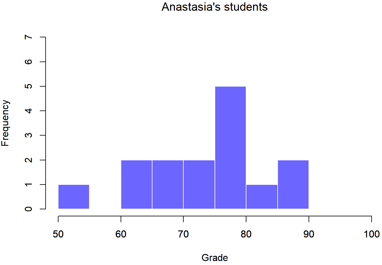
Anastasia’s students	74.53	9.00	15
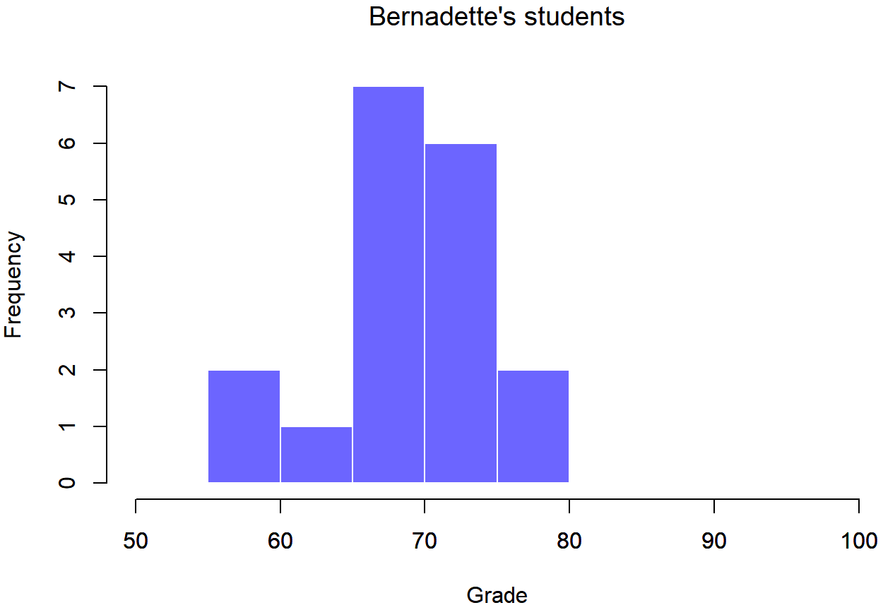
Bernadette’s students	69.06	5.77	18

To give you a more detailed sense of what’s going on here, I’ve plotted histograms showing the distribution of grades for both tutors (Figure 13.6 and 13.7). Inspection of these histograms suggests that the students in Anastasia’s class may be getting slightly better grades on average, though they also seem a little more variable.

Figure 13.6: Histogram showing the overall distribution of grades for students in Anastasia’s class

Figure 13.7: Histogram showing the overall distribution of grades for students in Bernadette’s class

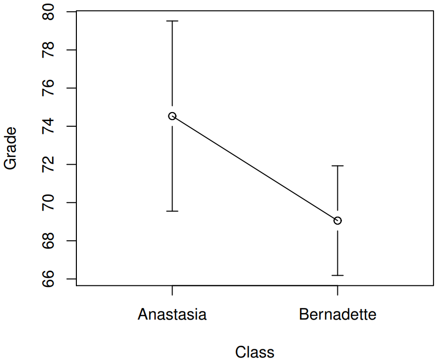
Here is a simpler plot showing the means and corresponding confidence intervals for both groups of students (Figure 13.8).

Figure 13.8: Plots showing the mean grade for the students in Anastasia’s and Bernadette’s tutorials. Error bars depict 95% confidence intervals around the mean. On the basis of visual inspection, it does look like there’s a real difference between the groups, though it’s hard to say for sure.

Introducing the test

The independent samples t-test comes in two different forms, Student’s and Welch’s. The original Student t-test – which is the one I’ll describe in this section – is the simpler of the two, but relies on much more restrictive assumptions than the Welch t-test. Assuming for the moment that you want to run a two-sided test, the goal is to determine whether two “independent samples” of data are drawn from populations with the same mean (the null hypothesis) or different means (the alternative hypothesis). When we say “independent” samples, what we really mean here is that there’s no special relationship between observations in the two samples. This probably doesn’t make a lot of sense right now, but it will be clearer when we come to talk about the paired samples t-test later on. For now, let’s just point out that if we have an experimental design where participants are randomly allocated to one of two groups, and we want to compare the two groups’ mean performance on some outcome measure, then an independent samples t-test (rather than a paired samples t-test) is what we’re after.

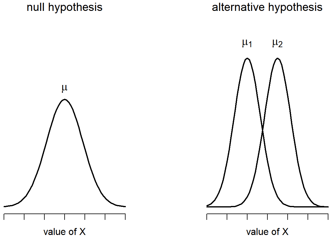
Okay, so let’s let μ₁ denote the true population mean for group 1 (e.g., Anastasia’s students), and μ₂ will be the true population mean for group 2 (e.g., Bernadette’s students),¹⁹⁰ and as usual we’ll let \(\bar{X}_{1}\) and \(\bar{X}_{2}\) denote the observed sample means for both of these groups. Our null hypothesis states that the two population means are identical (μ₁=μ₂) and the alternative to this is that they are not (μ₁≠μ₂). Written in mathematical-ese, this is…

H₀:μ₁=μ₂

H₁:μ₁≠μ₂

Figure 13.9: Graphical illustration of the null and alternative hypotheses assumed by the Student t-test. The null hypothesis assumes that both groups have the same mean μ, whereas the alternative assumes that they have different means μ₁ and μ₂. Notice that it is assumed that the population distributions are normal, and that, although the alternative hypothesis allows the group to have different means, it assumes they have the same standard deviation

To construct a hypothesis test that handles this scenario, we start by noting that if the null hypothesis is true, then the difference between the population means is exactly zero, μ₁−μ₂=0 As a consequence, a diagnostic test statistic will be based on the difference between the two sample means. Because if the null hypothesis is true, then we’d expect

\(\bar{X}_{1}\) - \(\bar{X}_{2}\)

to be pretty close to zero. However, just like we saw with our one-sample tests (i.e., the one-sample z-test and the one-sample t-test) we have to be precise about exactly how close to zero this difference

\(\ t ={\bar{X}_1 - \bar{X}_2 \over SE}\)

We just need to figure out what this standard error estimate actually is. This is a bit trickier than was the case for either of the two tests we’ve looked at so far, so we need to go through it a lot more carefully to understand how it works.

“pooled estimate” of the standard deviation

In the original “Student t-test”, we make the assumption that the two groups have the same population standard deviation: that is, regardless of whether the population means are the same, we assume that the population standard deviations are identical, σ₁=σ₂. Since we’re assuming that the two standard deviations are the same, we drop the subscripts and refer to both of them as σ. How should we estimate this? How should we construct a single estimate of a standard deviation when we have two samples? The answer is, basically, we average them. Well, sort of. Actually, what we do is take a weighed average of the variance estimates, which we use as our pooled estimate of the variance. The weight assigned to each sample is equal to the number of observations in that sample, minus 1. Mathematically, we can write this as

\(\ \omega_{1}\)=N₁−1

\(\ \omega_{2}\)=N₂−1

Now that we’ve assigned weights to each sample, we calculate the pooled estimate of the variance by taking the weighted average of the two variance estimates, \(\ \hat{\sigma_1}^2\) and \(\ \hat{\sigma_2}^2\)

\(\ \hat{\sigma_p}^2 ={ \omega_{1}\hat{\sigma_1}^2+\omega_{2}\hat{\sigma_2}^2 \over \omega_{1}+\omega_{2}}\)

Finally, we convert the pooled variance estimate to a pooled standard deviation estimate, by taking the square root. This gives us the following formula for \(\ \hat{\sigma_p}\),

\(\ \hat{\sigma_p} =\sqrt{\omega_1\hat{\sigma_1}^2+\omega_2\hat{\sigma_2}^2\over \omega_1+\omega_2} \)

And if you mentally substitute \(\ \omega_1\)=N1−1 and \(\ \omega_2\)=N2−1 into this equation you get a very ugly looking formula; a very ugly formula that actually seems to be the “standard” way of describing the pooled standard deviation estimate. It’s not my favourite way of thinking about pooled standard deviations, however.¹⁹¹

same pooled estimate, described differently

I prefer to think about it like this. Our data set actually corresponds to a set of N observations, which are sorted into two groups. So let’s use the notation X_ik to refer to the grade received by the i-th student in the k-th tutorial group: that is, X₁₁ is the grade received by the first student in Anastasia’s class, X₂₁ is her second student, and so on. And we have two separate group means \(\ \bar{X_1}\) and \(\ \bar{X_2}\), which we could “generically” refer to using the notation \(\ \bar{X_k}\), i.e., the mean grade for the k-th tutorial group. So far, so good. Now, since every single student falls into one of the two tutorials, and so we can describe their deviation from the group mean as the difference

\(\ X_{ik} - \bar{X_k}\)

So why not just use these deviations (i.e., the extent to which each student’s grade differs from the mean grade in their tutorial?) Remember, a variance is just the average of a bunch of squared deviations, so let’s do that. Mathematically, we could write it like this:

\(\ ∑_{ik} (X_{ik}-\bar{X}_k)^2 \over N \)

where the notation “∑_ik” is a lazy way of saying “calculate a sum by looking at all students in all tutorials”, since each “ik” corresponds to one student.¹⁹² But, as we saw in Chapter 10, calculating the variance by dividing by N produces a biased estimate of the population variance. And previously, we needed to divide by N−1 to fix this. However, as I mentioned at the time, the reason why this bias exists is because the variance estimate relies on the sample mean; and to the extent that the sample mean isn’t equal to the population mean, it can systematically bias our estimate of the variance. But this time we’re relying on two sample means! Does this mean that we’ve got more bias? Yes, yes it does. And does this mean we now need to divide by N−2 instead of N−1, in order to calculate our pooled variance estimate? Why, yes…

\(\hat{\sigma}_{p}\ ^{2}=\dfrac{\sum_{i k}\left(X_{i k}-X_{k}\right)^{2}}{N-2}\)

Oh, and if you take the square root of this then you get \(\ \hat{\sigma_{P}}\), the pooled standard deviation estimate. In other words, the pooled standard deviation calculation is nothing special: it’s not terribly different to the regular standard deviation calculation.

Completing the test

Regardless of which way you want to think about it, we now have our pooled estimate of the standard deviation. From now on, I’ll drop the silly p subscript, and just refer to this estimate as \(\ \hat{\sigma}\). Great. Let’s now go back to thinking about the bloody hypothesis test, shall we? Our whole reason for calculating this pooled estimate was that we knew it would be helpful when calculating our standard error estimate. But, standard error of what? In the one-sample t-test, it was the standard error of the sample mean, SE (\(\ \bar{X}\)), and since SE (\(\ \bar{X}=\sigma/ \sqrt{N}\) that’s what the denominator of our t-statistic looked like. This time around, however, we have two sample means. And what we’re interested in, specifically, is the the difference between the two \(\ \bar{X_1}\) - \(\ \bar{X_2}\). As a consequence, the standard error that we need to divide by is in fact the standard error of the difference between means. As long as the two variables really do have the same standard deviation, then our estimate for the standard error is

\(\operatorname{SE}\left(\bar{X}_{1}-\bar{X}_{2}\right)=\hat{\sigma} \sqrt{\dfrac{1}{N_{1}}+\dfrac{1}{N_{2}}}\)

and our t-statistic is therefore

\(t=\dfrac{\bar{X}_{1}-\bar{X}_{2}}{\operatorname{SE}\left(\bar{X}_{1}-\bar{X}_{2}\right)}\)

(shocking, isn’t it?) as long as the null hypothesis is true, and all of the assumptions of the test are met. The degrees of freedom, however, is slightly different. As usual, we can think of the degrees of freedom to be equal to the number of data points minus the number of constraints. In this case, we have N observations (N1 in sample 1, and N2 in sample 2), and 2 constraints (the sample means). So the total degrees of freedom for this test are N−2.

Doing the test in R

Not surprisingly, you can run an independent samples t-test using the t.test() function (Section 13.7), but once again I’m going to start with a somewhat simpler function in the lsr package. That function is unimaginatively called independentSamplesTTest(). First, recall that our data look like this:

head( harpo )

##   grade      tutor
## 1    65  Anastasia
## 2    72 Bernadette
## 3    66 Bernadette
## 4    74  Anastasia
## 5    73  Anastasia
## 6    71 Bernadette

The outcome variable for our test is the student grade, and the groups are defined in terms of the tutor for each class. So you probably won’t be too surprised to see that we’re going to describe the test that we want in terms of an R formula that reads like this grade ~ tutor. The specific command that we need is:

independentSamplesTTest( 
      formula = grade ~ tutor,  # formula specifying outcome and group variables
      data = harpo,             # data frame that contains the variables
      var.equal = TRUE          # assume that the two groups have the same variance
  )

## 
##    Student's independent samples t-test 
## 
## Outcome variable:   grade 
## Grouping variable:  tutor 
## 
## Descriptive statistics: 
##             Anastasia Bernadette
##    mean        74.533     69.056
##    std dev.     8.999      5.775
## 
## Hypotheses: 
##    null:        population means equal for both groups
##    alternative: different population means in each group
## 
## Test results: 
##    t-statistic:  2.115 
##    degrees of freedom:  31 
##    p-value:  0.043 
## 
## Other information: 
##    two-sided 95% confidence interval:  [0.197, 10.759] 
##    estimated effect size (Cohen's d):  0.74

The first two arguments should be familiar to you. The first one is the formula that tells R what variables to use and the second one tells R the name of the data frame that stores those variables. The third argument is not so obvious. By saying var.equal = TRUE, what we’re really doing is telling R to use the Student independent samples t-test. More on this later. For now, lets ignore that bit and look at the output:

The output has a very familiar form. First, it tells you what test was run, and it tells you the names of the variables that you used. The second part of the output reports the sample means and standard deviations for both groups (i.e., both tutorial groups). The third section of the output states the null hypothesis and the alternative hypothesis in a fairly explicit form. It then reports the test results: just like last time, the test results consist of a t-statistic, the degrees of freedom, and the p-value. The final section reports two things: it gives you a confidence interval, and an effect size. I’ll talk about effect sizes later. The confidence interval, however, I should talk about now.

It’s pretty important to be clear on what this confidence interval actually refers to: it is a confidence interval for the difference between the group means. In our example, Anastasia’s students had an average grade of 74.5, and Bernadette’s students had an average grade of 69.1, so the difference between the two sample means is 5.4. But of course the difference between population means might be bigger or smaller than this. The confidence interval reported by the independentSamplesTTest() function tells you that there’s a 95% chance that the true difference between means lies between 0.2 and 10.8.

In any case, the difference between the two groups is significant (just barely), so we might write up the result using text like this:

The mean grade in Anastasia’s class was 74.5% (std dev = 9.0), whereas the mean in Bernadette’s class was 69.1% (std dev = 5.8). A Student’s independent samples t-test showed that this 5.4% difference was significant (t(31)=2.1, p<.05, CI₉₅=[0.2,10.8], d=.74), suggesting that a genuine difference in learning outcomes has occurred.

Notice that I’ve included the confidence interval and the effect size in the stat block. People don’t always do this. At a bare minimum, you’d expect to see the t-statistic, the degrees of freedom and the p value. So you should include something like this at a minimum: t(31)=2.1, p<.05. If statisticians had their way, everyone would also report the confidence interval and probably the effect size measure too, because they are useful things to know. But real life doesn’t always work the way statisticians want it to: you should make a judgment based on whether you think it will help your readers, and (if you’re writing a scientific paper) the editorial standard for the journal in question. Some journals expect you to report effect sizes, others don’t. Within some scientific communities it is standard practice to report confidence intervals, in other it is not. You’ll need to figure out what your audience expects. But, just for the sake of clarity, if you’re taking my class: my default position is that it’s usually worth includng the effect size, but don’t worry about the confidence interval unless the assignment asks you to or implies that you should.

Positive and negative t values

Before moving on to talk about the assumptions of the t-test, there’s one additional point I want to make about the use of t-tests in practice. The first one relates to the sign of the t-statistic (that is, whether it is a positive number or a negative one). One very common worry that students have when they start running their first t-test is that they often end up with negative values for the t-statistic, and don’t know how to interpret it. In fact, it’s not at all uncommon for two people working independently to end up with R outputs that are almost identical, except that one person has a negative t values and the other one has a positive t value. Assuming that you’re running a two-sided test, then the p-values will be identical. On closer inspection, the students will notice that the confidence intervals also have the opposite signs. This is perfectly okay: whenever this happens, what you’ll find is that the two versions of the R output arise from slightly different ways of running the t-test. What’s happening here is very simple. The t-statistic that R is calculating here is always of the form

\(t=\dfrac{(\text { mean } 1)-(\text { mean } 2)}{(\mathrm{SE})}\)

If “mean 1” is larger than “mean 2” the t statistic will be positive, whereas if “mean 2” is larger then the t statistic will be negative. Similarly, the confidence interval that R reports is the confidence interval for the difference “(mean 1) minus (mean 2)”, which will be the reverse of what you’d get if you were calculating the confidence interval for the difference “(mean 2) minus (mean 1)”.

Okay, that’s pretty straightforward when you think about it, but now consider our t-test comparing Anastasia’s class to Bernadette’s class. Which one should we call “mean 1” and which one should we call “mean 2”. It’s arbitrary. However, you really do need to designate one of them as “mean 1” and the other one as “mean 2”. Not surprisingly, the way that R handles this is also pretty arbitrary. In earlier versions of the book I used to try to explain it, but after a while I gave up, because it’s not really all that important, and to be honest I can never remember myself. Whenever I get a significant t-test result, and I want to figure out which mean is the larger one, I don’t try to figure it out by looking at the t-statistic. Why would I bother doing that? It’s foolish. It’s easier just look at the actual group means, since the R output actually shows them!

Here’s the important thing. Because it really doesn’t matter what R printed out, I usually try to report the t-statistic in such a way that the numbers match up with the text. Here’s what I mean… suppose that what I want to write in my report is “Anastasia’s class had higher grades than Bernadette’s class”. The phrasing here implies that Anastasia’s group comes first, so it makes sense to report the t-statistic as if Anastasia’s class corresponded to group 1. If so, I would write

Anastasia’s class had higher grades than Bernadette’s class (t(31)=2.1,p=.04).

(I wouldn’t actually emphasise the word “higher” in real life, I’m just doing it to emphasise the point that “higher” corresponds to positive t values). On the other hand, suppose the phrasing I wanted to use has Bernadette’s class listed first. If so, it makes more sense to treat her class as group 1, and if so, the write up looks like this:

Bernadette’s class had lower grades than Anastasia’s class (t(31)=−2.1,p=.04).

Because I’m talking about one group having “lower” scores this time around, it is more sensible to use the negative form of the t-statistic. It just makes it read more cleanly.

One last thing: please note that you can’t do this for other types of test statistics. It works for t-tests, but it wouldn’t be meaningful for chi-square testsm F-tests or indeed for most of the tests I talk about in this book. So don’t overgeneralise this advice! I’m really just talking about t-tests here and nothing else!

Assumptions of the test

As always, our hypothesis test relies on some assumptions. So what are they? For the Student t-test there are three assumptions, some of which we saw previously in the context of the one sample t-test (see Section 13.2.3):

• Normality. Like the one-sample t-test, it is assumed that the data are normally distributed. Specifically, we assume that both groups are normally distributed. In Section 13.9 we’ll discuss how to test for normality, and in Section 13.10 we’ll discuss possible solutions.
• Independence. Once again, it is assumed that the observations are independently sampled. In the context of the Student test this has two aspects to it. Firstly, we assume that the observations within each sample are independent of one another (exactly the same as for the one-sample test). However, we also assume that there are no cross-sample dependencies. If, for instance, it turns out that you included some participants in both experimental conditions of your study (e.g., by accidentally allowing the same person to sign up to different conditions), then there are some cross sample dependencies that you’d need to take into account.
• Homogeneity of variance (also called “homoscedasticity”). The third assumption is that the population standard deviation is the same in both groups. You can test this assumption using the Levene test, which I’ll talk about later on in the book (Section 14.7). However, there’s a very simple remedy for this assumption, which I’ll talk about in the next section.