5.2: Measures of Variability

Last updated
Save as PDF

Page ID: 3966

$ \newcommand{\vecs}[1]{\overset { \scriptstyle \rightharpoonup} {\mathbf{#1}} } $ $ \newcommand{\vecd}[1]{\overset{-\!-\!\rightharpoonup}{\vphantom{a}\smash {#1}}} $$\newcommand{\id}{\mathrm{id}}$ $ \newcommand{\Span}{\mathrm{span}}$ $ \newcommand{\kernel}{\mathrm{null}\,}$ $ \newcommand{\range}{\mathrm{range}\,}$ $ \newcommand{\RealPart}{\mathrm{Re}}$ $ \newcommand{\ImaginaryPart}{\mathrm{Im}}$ $ \newcommand{\Argument}{\mathrm{Arg}}$ $ \newcommand{\norm}[1]{\| #1 \|}$ $ \newcommand{\inner}[2]{\langle #1, #2 \rangle}$ $ \newcommand{\Span}{\mathrm{span}}$ $\newcommand{\id}{\mathrm{id}}$ $ \newcommand{\Span}{\mathrm{span}}$ $ \newcommand{\kernel}{\mathrm{null}\,}$ $ \newcommand{\range}{\mathrm{range}\,}$ $ \newcommand{\RealPart}{\mathrm{Re}}$ $ \newcommand{\ImaginaryPart}{\mathrm{Im}}$ $ \newcommand{\Argument}{\mathrm{Arg}}$ $ \newcommand{\norm}[1]{\| #1 \|}$ $ \newcommand{\inner}[2]{\langle #1, #2 \rangle}$ $ \newcommand{\Span}{\mathrm{span}}$$\newcommand{\AA}{\unicode[.8,0]{x212B}}$

The statistics that we’ve discussed so far all relate to central tendency. That is, they all talk about which values are “in the middle” or “popular” in the data. However, central tendency is not the only type of summary statistic that we want to calculate. The second thing that we really want is a measure of the variability of the data. That is, how “spread out” are the data? How “far” away from the mean or median do the observed values tend to be? For now, let’s assume that the data are interval or ratio scale, so we’ll continue to use the afl.margins data. We’ll use this data to discuss several different measures of spread, each with different strengths and weaknesses.

Range

The range of a variable is very simple: it’s the biggest value minus the smallest value. For the AFL winning margins data, the maximum value is 116, and the minimum value is 0. We can calculate these values in R using the max() and min() functions:

max( afl.margins )

## [1] 116

min( afl.margins )

## [1] 0

where I’ve omitted the output because it’s not interesting. The other possibility is to use the range() function; which outputs both the minimum value and the maximum value in a vector, like this:

range( afl.margins )

## [1]   0 116

Although the range is the simplest way to quantify the notion of “variability”, it’s one of the worst. Recall from our discussion of the mean that we want our summary measure to be robust. If the data set has one or two extremely bad values in it, we’d like our statistics not to be unduly influenced by these cases. If we look once again at our toy example of a data set containing very extreme outliers…

−100,2,3,4,5,6,7,8,9,10

… it is clear that the range is not robust, since this has a range of 110, but if the outlier were removed we would have a range of only 8.

Interquartile range

The interquartile range (IQR) is like the range, but instead of calculating the difference between the biggest and smallest value, it calculates the difference between the 25th quantile and the 75th quantile. Probably you already know what a quantile is (they’re more commonly called percentiles), but if not: the 10th percentile of a data set is the smallest number x such that 10% of the data is less than x. In fact, we’ve already come across the idea: the median of a data set is its 50th quantile / percentile! R actually provides you with a way of calculating quantiles, using the (surprise, surprise) quantile() function. Let’s use it to calculate the median AFL winning margin:

quantile( x = afl.margins, probs = .5)

##  50% 
## 30.5

And not surprisingly, this agrees with the answer that we saw earlier with the median() function. Now, we can actually input lots of quantiles at once, by specifying a vector for the probs argument. So lets do that, and get the 25th and 75th percentile:

quantile( x = afl.margins, probs = c(.25,.75) )

##   25%   75% 
## 12.75 50.50

And, by noting that 50.5−12.75=37.75, we can see that the interquartile range for the 2010 AFL winning margins data is 37.75. Of course, that seems like too much work to do all that typing, so R has a built in function called IQR() that we can use:

IQR( x = afl.margins )

## [1] 37.75

While it’s obvious how to interpret the range, it’s a little less obvious how to interpret the IQR. The simplest way to think about it is like this: the interquartile range is the range spanned by the “middle half” of the data. That is, one quarter of the data falls below the 25th percentile, one quarter of the data is above the 75th percentile, leaving the “middle half” of the data lying in between the two. And the IQR is the range covered by that middle half.

Mean absolute deviation

The two measures we’ve looked at so far, the range and the interquartile range, both rely on the idea that we can measure the spread of the data by looking at the quantiles of the data. However, this isn’t the only way to think about the problem. A different approach is to select a meaningful reference point (usually the mean or the median) and then report the “typical” deviations from that reference point. What do we mean by “typical” deviation? Usually, the mean or median value of these deviations! In practice, this leads to two different measures, the “mean absolute deviation (from the mean)” and the “median absolute deviation (from the median)”. From what I’ve read, the measure based on the median seems to be used in statistics, and does seem to be the better of the two, but to be honest I don’t think I’ve seen it used much in psychology. The measure based on the mean does occasionally show up in psychology though. In this section I’ll talk about the first one, and I’ll come back to talk about the second one later.

Since the previous paragraph might sound a little abstract, let’s go through the mean absolute deviation from the mean a little more slowly. One useful thing about this measure is that the name actually tells you exactly how to calculate it. Let’s think about our AFL winning margins data, and once again we’ll start by pretending that there’s only 5 games in total, with winning margins of 56, 31, 56, 8 and 32. Since our calculations rely on an examination of the deviation from some reference point (in this case the mean), the first thing we need to calculate is the mean, $\bar{X}$. For these five observations, our mean is $\bar{X}$=36.6. The next step is to convert each of our observations X_i into a deviation score. We do this by calculating the difference between the observation Xi and the mean $\bar{X}$. That is, the deviation score is defined to be X_i−$\bar{X}$. For the first observation in our sample, this is equal to 56−36.6=19.4. Okay, that’s simple enough. The next step in the process is to convert these deviations to absolute deviations. As we discussed earlier when talking about the abs() function in R (Section 3.5), we do this by converting any negative values to positive ones. Mathematically, we would denote the absolute value of −3 as |−3|, and so we say that |−3|=3. We use the absolute value function here because we don’t really care whether the value is higher than the mean or lower than the mean, we’re just interested in how close it is to the mean. To help make this process as obvious as possible, the table below shows these calculations for all five observations:

the observation	its symbol	the observed value
winning margin, game 2	X2	31 points
winning margin, game 5	X5	32 points
winning margin, game 1	X1	56 points
winning margin, game 3	X3	56 points
winning margin, game 4	X4	8 points

Now that we have calculated the absolute deviation score for every observation in the data set, all that we have to do to calculate the mean of these scores. Let’s do that:

\[
\dfrac{19.4+5.6+19.4+28.6+4.6}{5}=15.52
\nonumber\]

And we’re done. The mean absolute deviation for these five scores is 15.52.

However, while our calculations for this little example are at an end, we do have a couple of things left to talk about. Firstly, we should really try to write down a proper mathematical formula. But in order do to this I need some mathematical notation to refer to the mean absolute deviation. Irritatingly, “mean absolute deviation” and “median absolute deviation” have the same acronym (MAD), which leads to a certain amount of ambiguity, and since R tends to use MAD to refer to the median absolute deviation, I’d better come up with something different for the mean absolute deviation. Sigh. What I’ll do is use AAD instead, short for average absolute deviation. Now that we have some unambiguous notation, here’s the formula that describes what we just calculated:

\[
(X)=\dfrac{1}{N} \sum_{i=1}^{N}\left|X_{i}-\bar{X}\right|
\nonumber\]

The last thing we need to talk about is how to calculate AAD in R. One possibility would be to do everything using low level commands, laboriously following the same steps that I used when describing the calculations above. However, that’s pretty tedious. You’d end up with a series of commands that might look like this:

X <- c(56, 31,56,8,32)   # enter the data
X.bar <- mean( X )       # step 1. the mean of the data
AD <- abs( X - X.bar )   # step 2. the absolute deviations from the mean
AAD <- mean( AD )        # step 3. the mean absolute deviations
print( AAD )             # print the results

## [1] 15.52

Each of those commands is pretty simple, but there’s just too many of them. And because I find that to be too much typing, the lsr package has a very simple function called aad() that does the calculations for you. If we apply the aad() function to our data, we get this:

library(lsr)
aad( X )

## [1] 15.52

No suprises there.

Variance

Although the mean absolute deviation measure has its uses, it’s not the best measure of variability to use. From a purely mathematical perspective, there are some solid reasons to prefer squared deviations rather than absolute deviations. If we do that, we obtain a measure is called the variance, which has a lot of really nice statistical properties that I’m going to ignore,⁷¹(X)$ and Var(Y) respectively. Now imagine I want to define a new variable Z that is the sum of the two, Z=X+Y. As it turns out, the variance of Z is equal to Var(X)+Var(Y). This is a very useful property, but it’s not true of the other measures that I talk about in this section.] and one massive psychological flaw that I’m going to make a big deal out of in a moment. The variance of a data set X is sometimes written as Var(X), but it’s more commonly denoted s² (the reason for this will become clearer shortly). The formula that we use to calculate the variance of a set of observations is as follows:

\[
\begin{aligned}
&\operatorname{Var}(X)=\dfrac{1}{N} \sum_{i=1}^{N}\left(X_{i}-\bar{X}\right)^{2}\\
&\operatorname{Var}(X)=\dfrac{\sum_{i=1}^{N}\left(X_{i}-\bar{X}\right)^{2}}{N}
\end{aligned}
\nonumber\]

As you can see, it’s basically the same formula that we used to calculate the mean absolute deviation, except that instead of using “absolute deviations” we use “squared deviations”. It is for this reason that the variance is sometimes referred to as the “mean square deviation”.

Now that we’ve got the basic idea, let’s have a look at a concrete example. Once again, let’s use the first five AFL games as our data. If we follow the same approach that we took last time, we end up with the following table:

Table 5.1: Basic arithmetic operations in R. These five operators are used very frequently throughout the text, so it’s important to be familiar with them at the outset.

i [which game]	X_i [value]	X_i−$\bar{X}$ [deviation from mean]	(Xi−$\bar{X}$)² [absolute deviation]
5	32	-4.6	21.16
2	31	-5.6	31.36
1	56	19.4	376.36
3	56	19.4	376.36
4	8	-28.6	817.96

That last column contains all of our squared deviations, so all we have to do is average them. If we do that by typing all the numbers into R by hand…

( 376.36 + 31.36 + 376.36 + 817.96 + 21.16 ) / 5

## [1] 324.64

… we end up with a variance of 324.64. Exciting, isn’t it? For the moment, let’s ignore the burning question that you’re all probably thinking (i.e., what the heck does a variance of 324.64 actually mean?) and instead talk a bit more about how to do the calculations in R, because this will reveal something very weird.

As always, we want to avoid having to type in a whole lot of numbers ourselves. And as it happens, we have the vector X lying around, which we created in the previous section. With this in mind, we can calculate the variance of X by using the following command,

mean( (X - mean(X) )^2)

## [1] 324.64

and as usual we get the same answer as the one that we got when we did everything by hand. However, I still think that this is too much typing. Fortunately, R has a built in function called var() which does calculate variances. So we could also do this…

var(X)

## [1] 405.8

and you get the same… no, wait… you get a completely different answer. That’s just weird. Is R broken? Is this a typo? Is Dan an idiot?

As it happens, the answer is no.⁷² It’s not a typo, and R is not making a mistake. To get a feel for what’s happening, let’s stop using the tiny data set containing only 5 data points, and switch to the full set of 176 games that we’ve got stored in our afl.margins vector. First, let’s calculate the variance by using the formula that I described above:

mean( (afl.margins - mean(afl.margins) )^2)

## [1] 675.9718

Now let’s use the var() function:

var( afl.margins )

## [1] 679.8345

Hm. These two numbers are very similar this time. That seems like too much of a coincidence to be a mistake. And of course it isn’t a mistake. In fact, it’s very simple to explain what R is doing here, but slightly trickier to explain why R is doing it. So let’s start with the “what”. What R is doing is evaluating a slightly different formula to the one I showed you above. Instead of averaging the squared deviations, which requires you to divide by the number of data points N, R has chosen to divide by N−1. In other words, the formula that R is using is this one

\[
\dfrac{1}{N-1} \sum_{i=1}^{N}\left(X_{i}-\bar{X}\right)^{2}
\nonumber\]

It’s easy enough to verify that this is what’s happening, as the following command illustrates:

sum( (X-mean(X))^2 ) / 4

## [1] 405.8

This is the same answer that R gave us originally when we calculated var(X) originally. So that’s the what. The real question is why R is dividing by N−1 and not by N. After all, the variance is supposed to be the mean squared deviation, right? So shouldn’t we be dividing by N, the actual number of observations in the sample? Well, yes, we should. However, as we’ll discuss in Chapter 10, there’s a subtle distinction between “describing a sample” and “making guesses about the population from which the sample came”. Up to this point, it’s been a distinction without a difference. Regardless of whether you’re describing a sample or drawing inferences about the population, the mean is calculated exactly the same way. Not so for the variance, or the standard deviation, or for many other measures besides. What I outlined to you initially (i.e., take the actual average, and thus divide by N) assumes that you literally intend to calculate the variance of the sample. Most of the time, however, you’re not terribly interested in the sample in and of itself. Rather, the sample exists to tell you something about the world. If so, you’re actually starting to move away from calculating a “sample statistic”, and towards the idea of estimating a “population parameter”. However, I’m getting ahead of myself. For now, let’s just take it on faith that R knows what it’s doing, and we’ll revisit the question later on when we talk about estimation in Chapter 10.

Okay, one last thing. This section so far has read a bit like a mystery novel. I’ve shown you how to calculate the variance, described the weird “N−1” thing that R does and hinted at the reason why it’s there, but I haven’t mentioned the single most important thing… how do you interpret the variance? Descriptive statistics are supposed to describe things, after all, and right now the variance is really just a gibberish number. Unfortunately, the reason why I haven’t given you the human-friendly interpretation of the variance is that there really isn’t one. This is the most serious problem with the variance. Although it has some elegant mathematical properties that suggest that it really is a fundamental quantity for expressing variation, it’s completely useless if you want to communicate with an actual human… variances are completely uninterpretable in terms of the original variable! All the numbers have been squared, and they don’t mean anything anymore. This is a huge issue. For instance, according to the table I presented earlier, the margin in game 1 was “376.36 points-squared higher than the average margin”. This is exactly as stupid as it sounds; and so when we calculate a variance of 324.64, we’re in the same situation. I’ve watched a lot of footy games, and never has anyone referred to “points squared”. It’s not a real unit of measurement, and since the variance is expressed in terms of this gibberish unit, it is totally meaningless to a human.

Standard deviation

Okay, suppose that you like the idea of using the variance because of those nice mathematical properties that I haven’t talked about, but – since you’re a human and not a robot – you’d like to have a measure that is expressed in the same units as the data itself (i.e., points, not points-squared). What should you do? The solution to the problem is obvious: take the square root of the variance, known as the standard deviation, also called the “root mean squared deviation”, or RMSD. This solves out problem fairly neatly: while nobody has a clue what “a variance of 324.68 points-squared” really means, it’s much easier to understand “a standard deviation of 18.01 points”, since it’s expressed in the original units. It is traditional to refer to the standard deviation of a sample of data as s, though “sd” and “std dev.” are also used at times. Because the standard deviation is equal to the square root of the variance, you probably won’t be surprised to see that the formula is:

\[
s=\sqrt{\dfrac{1}{N} \sum_{i=1}^{N}\left(X_{i}-\bar{X}\right)^{2}}
\nonumber\]

and the R function that we use to calculate it is sd(). However, as you might have guessed from our discussion of the variance, what R actually calculates is slightly different to the formula given above. Just like the we saw with the variance, what R calculates is a version that divides by N−1 rather than N. For reasons that will make sense when we return to this topic in Chapter@refch:estimation I’ll refer to this new quantity as $\hat{\sigma}$ (read as: “sigma hat”), and the formula for this is

\[
\hat{\sigma}=\sqrt{\dfrac{1}{N-1} \sum_{i=1}^{N}\left(X_{i}-\bar{X}\right)^{2}}
\nonumber\]

With that in mind, calculating standard deviations in R is simple:

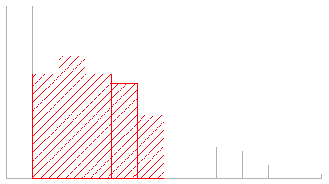
sd( afl.margins )

## [1] 26.07364

Interpreting standard deviations is slightly more complex. Because the standard deviation is derived from the variance, and the variance is a quantity that has little to no meaning that makes sense to us humans, the standard deviation doesn’t have a simple interpretation. As a consequence, most of us just rely on a simple rule of thumb: in general, you should expect 68% of the data to fall within 1 standard deviation of the mean, 95% of the data to fall within 2 standard deviation of the mean, and 99.7% of the data to fall within 3 standard deviations of the mean. This rule tends to work pretty well most of the time, but it’s not exact: it’s actually calculated based on an assumption that the histogram is symmetric and “bell shaped.”⁷³ As you can tell from looking at the AFL winning margins histogram in Figure 5.1, this isn’t exactly true of our data! Even so, the rule is approximately correct. As it turns out, 65.3% of the AFL margins data fall within one standard deviation of the mean. This is shown visually in Figure 5.3.

Figure 5.3: An illustration of the standard deviation, applied to the AFL winning margins data. The shaded bars in the histogram show how much of the data fall within one standard deviation of the mean. In this case, 65.3% of the data set lies within this range, which is pretty consistent with the “approximately 68% rule” discussed in the main text.

Median absolute deviation

The last measure of variability that I want to talk about is the median absolute deviation (MAD). The basic idea behind MAD is very simple, and is pretty much identical to the idea behind the mean absolute deviation (Section 5.2.3). The difference is that you use the median everywhere. If we were to frame this idea as a pair of R commands, they would look like this:

# mean absolute deviation from the mean:
mean( abs(afl.margins - mean(afl.margins)) )

## [1] 21.10124

# *median* absolute deviation from the *median*:
median( abs(afl.margins - median(afl.margins)) )

## [1] 19.5

This has a straightforward interpretation: every observation in the data set lies some distance away from the typical value (the median). So the MAD is an attempt to describe a typical deviation from a typical value in the data set. It wouldn’t be unreasonable to interpret the MAD value of 19.5 for our AFL data by saying something like this:

The median winning margin in 2010 was 30.5, indicating that a typical game involved a winning margin of about 30 points. However, there was a fair amount of variation from game to game: the MAD value was 19.5, indicating that a typical winning margin would differ from this median value by about 19-20 points.

As you’d expect, R has a built in function for calculating MAD, and you will be shocked no doubt to hear that it’s called mad(). However, it’s a little bit more complicated than the functions that we’ve been using previously. If you want to use it to calculate MAD in the exact same way that I have described it above, the command that you need to use specifies two arguments: the data set itself x, and a constant that I’ll explain in a moment. For our purposes, the constant is 1, so our command becomes

mad( x = afl.margins, constant = 1 )

## [1] 19.5

Apart from the weirdness of having to type that constant = 1 part, this is pretty straightforward.

Okay, so what exactly is this constant = 1 argument? I won’t go into all the details here, but here’s the gist. Although the “raw” MAD value that I’ve described above is completely interpretable on its own terms, that’s not actually how it’s used in a lot of real world contexts. Instead, what happens a lot is that the researcher actually wants to calculate the standard deviation. However, in the same way that the mean is very sensitive to extreme values, the standard deviation is vulnerable to the exact same issue. So, in much the same way that people sometimes use the median as a “robust” way of calculating “something that is like the mean”, it’s not uncommon to use MAD as a method for calculating “something that is like the standard deviation”. Unfortunately, the raw MAD value doesn’t do this. Our raw MAD value is 19.5, and our standard deviation was 26.07. However, what some clever person has shown is that, under certain assumptions⁷⁴, you can multiply the raw MAD value by 1.4826 and obtain a number that is directly comparable to the standard deviation. As a consequence, the default value of constant is 1.4826, and so when you use the mad() command without manually setting a value, here’s what you get:

mad( afl.margins )

## [1] 28.9107

I should point out, though, that if you want to use this “corrected” MAD value as a robust version of the standard deviation, you really are relying on the assumption that the data are (or at least, are “supposed to be” in some sense) symmetric and basically shaped like a bell curve. That’s really not true for our afl.margins data, so in this case I wouldn’t try to use the MAD value this way.

Which measure to use?

We’ve discussed quite a few measures of spread (range, IQR, MAD, variance and standard deviation), and hinted at their strengths and weaknesses. Here’s a quick summary:

Range. Gives you the full spread of the data. It’s very vulnerable to outliers, and as a consequence it isn’t often used unless you have good reasons to care about the extremes in the data.
Interquartile range. Tells you where the “middle half” of the data sits. It’s pretty robust, and complements the median nicely. This is used a lot.
Mean absolute deviation. Tells you how far “on average” the observations are from the mean. It’s very interpretable, but has a few minor issues (not discussed here) that make it less attractive to statisticians than the standard deviation. Used sometimes, but not often.
Variance. Tells you the average squared deviation from the mean. It’s mathematically elegant, and is probably the “right” way to describe variation around the mean, but it’s completely uninterpretable because it doesn’t use the same units as the data. Almost never used except as a mathematical tool; but it’s buried “under the hood” of a very large number of statistical tools.
Standard deviation. This is the square root of the variance. It’s fairly elegant mathematically, and it’s expressed in the same units as the data so it can be interpreted pretty well. In situations where the mean is the measure of central tendency, this is the default. This is by far the most popular measure of variation.
Median absolute deviation. The typical (i.e., median) deviation from the median value. In the raw form it’s simple and interpretable; in the corrected form it’s a robust way to estimate the standard deviation, for some kinds of data sets. Not used very often, but it does get reported sometimes.

In short, the IQR and the standard deviation are easily the two most common measures used to report the variability of the data; but there are situations in which the others are used. I’ve described all of them in this book because there’s a fair chance you’ll run into most of these somewhere.