9.1: Factorial Basics

Last updated
Save as PDF

Page ID: 7940

\( \newcommand{\vecs}[1]{\overset { \scriptstyle \rightharpoonup} {\mathbf{#1}} } \) \( \newcommand{\vecd}[1]{\overset{-\!-\!\rightharpoonup}{\vphantom{a}\smash {#1}}} \)\(\newcommand{\id}{\mathrm{id}}\) \( \newcommand{\Span}{\mathrm{span}}\) \( \newcommand{\kernel}{\mathrm{null}\,}\) \( \newcommand{\range}{\mathrm{range}\,}\) \( \newcommand{\RealPart}{\mathrm{Re}}\) \( \newcommand{\ImaginaryPart}{\mathrm{Im}}\) \( \newcommand{\Argument}{\mathrm{Arg}}\) \( \newcommand{\norm}[1]{\| #1 \|}\) \( \newcommand{\inner}[2]{\langle #1, #2 \rangle}\) \( \newcommand{\Span}{\mathrm{span}}\) \(\newcommand{\id}{\mathrm{id}}\) \( \newcommand{\Span}{\mathrm{span}}\) \( \newcommand{\kernel}{\mathrm{null}\,}\) \( \newcommand{\range}{\mathrm{range}\,}\) \( \newcommand{\RealPart}{\mathrm{Re}}\) \( \newcommand{\ImaginaryPart}{\mathrm{Im}}\) \( \newcommand{\Argument}{\mathrm{Arg}}\) \( \newcommand{\norm}[1]{\| #1 \|}\) \( \newcommand{\inner}[2]{\langle #1, #2 \rangle}\) \( \newcommand{\Span}{\mathrm{span}}\)\(\newcommand{\AA}{\unicode[.8,0]{x212B}}\)

2x2 Designs

We’ve just started talking about a 2x2 Factorial design. We said this means the IVs are crossed. To illustrate this, take a look at the following tables. We show an abstract version and a concrete version using time of day and caffeine as the two IVs, each with two levels in the design:

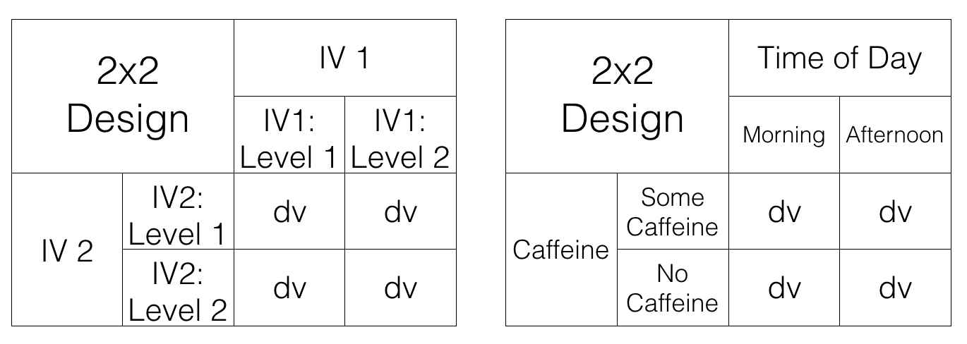
2x2 factorial design structure. — Figure \(\PageIndex{1}\): Structure of 2x2 factorial designs.

Let’s talk about this crossing business. Here’s what it means for the design. For the first level of Time of Day (morning), we measure test performance when some people drank caffeine and some did not. So, in the morning we manipulate whether or not caffeine is taken. Also, in the second level of the Time of Day (afternoon), we also manipulate caffeine. Some people drink or don’t drink caffeine in the afternoon as well, and we collect measures of test performance in both conditions.

We could say the same thing, but talk from the point of view of the second IV. For example, when people drink caffeine, we test those people in the morning, and in the afternoon. So, time of day is manipulated for the people who drank caffeine. Also, when people do not drink caffeine, we test those people in the morning, and in the afternoon, So, time of day is manipulated for the people who did not drink caffeine.

Finally, each of the four squares representing a DV, is called a condition. So, we have 2 IVs, each with 2 levels, for a total of 4 conditions. This is why we call it a 2x2 design. 2x2 = 4. The notation tells us how to calculate the total number of conditions.

Factorial Notation

Anytime all of the levels of each IV in a design are fully crossed, so that they all occur for each level of every other IV, we can say the design is a fully factorial design.

We use a notation system to refer to these designs. The rules for notation are as follows. Each IV get’s it’s own number. The number of levels in the IV is the number we use for the IV. Let’s look at some examples:

2x2 = There are two IVS, the first IV has two levels, the second IV has 2 levels. There are a total of 4 conditions, 2x2 = 4.

2x3 = There are two IVs, the first IV has two levels, the second IV has three levels. There are a total of 6 conditions, 2x3 = 6

3x2 = There are two IVs, the first IV has three levels, the second IV has two levels. There are a total of 6 conditions, 3x2=6.

4x4 = There are two IVs, the first IV has 4 levels, the second IV has 4 levels. There are a total of 16 condition, 4x4=16

2x3x2 = There are a total of three IVs. The first IV has 2 levels. The second IV has 3 levels. The third IV has 2 levels. There are a total of 12 condition. 2x3x2 = 12.

2 x 3 designs

Just for fun, let’s illustrate a 2x3 design using the same kinds of tables we looked at before for the 2x2 design.

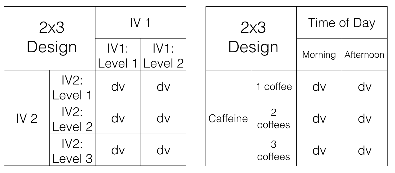
2x3 factorial design structure. — Figure \(\PageIndex{2}\): Structure of 2x3 factorial design.

All we did was add another row for the second IV. It’s a 2x3 design, so it should have 6 conditions. As you can see there are now 6 cells to measure the DV.