14.1: Dummy Variables

Thus far, we have considered OLS models that include variables measured on interval level scales (or, in a pinch and with caution, ordinal scales). That is fine when we have variables for which we can develop valid and reliable interval (or ordinal) measures. But in the policy and social science worlds, we often want to include in our analysis concepts that do not readily admit to interval measure – including many cases in which a variable has an “on - off”, or “present - absent” quality. In other cases we want to include a concept that is essentially nominal in nature, such that an observation can be categorized as a subset but not measured on a “high-low” or “more-less” type of scale. In these instances we can utilize what is generally known as a dummy variable, but are also referred to as indicator variables, Boolean variables, or categorical variables.

What the Heck are “Dummy Variables”?

• A dichotomous variable, with values of 0 and 1;
• A value of 1 represents the presence of some quality, a zero its absence;
• The 1s are compared to the 0s, who are known as the referent group“;
• Dummy variables are often thought of as a proxy for a qualitative variable.

Dummy variables allow for tests of the differences in overall value of the YY for different nominal groups in the data. They are akin to a difference of means test for the groups identified by the dummy variable. Dummy variables allow for comparisons between an included (the 1s) and an omitted (the 0s) group. Therefore, it is important to be clear about which group is omitted and serving as the comparison category."

It is often the case that there are more than two groups represented by a set of nominal categories. In that case, the variable will consist of two or more dummy variables, with 0/1 codes for each category except the referent group (which is omitted). Several examples of categorical variables that can be represented in multiple regression with dummy variables include:

• Experimental treatment and control groups (treatment=1, control=0)
• Gender (male=1, female=0 or vice versa)
• Race and ethnicity (a dummy for each group, with one omitted referent group)
• Region of residence (dummy for each region with one omitted reference region)
• Type of education (dummy for each type with omitted reference type)
• Religious affiliation (dummy for each religious denomination with omitted reference)

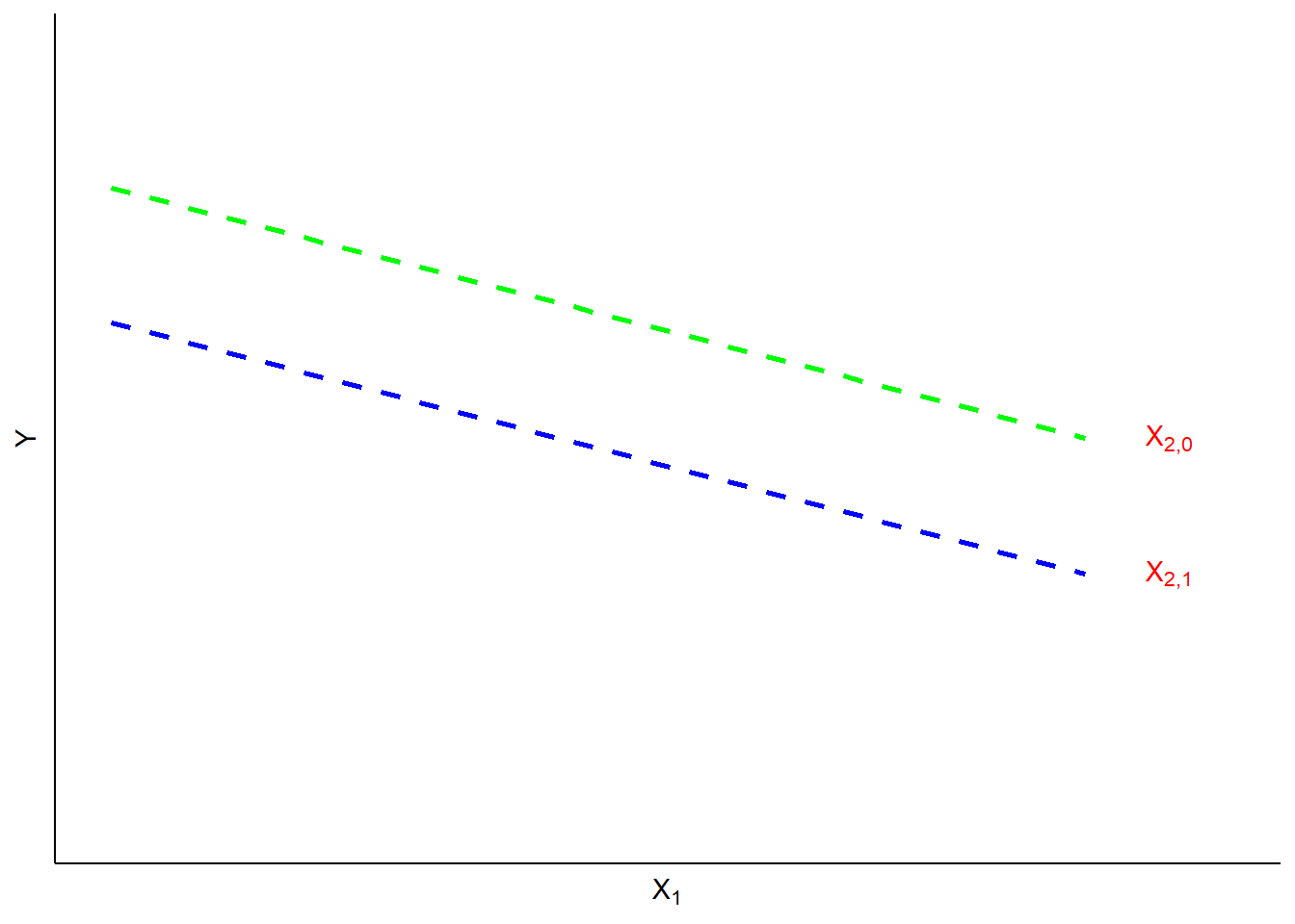
The value of the dummy coefficient represents the estimated difference in YY between the dummy group and the reference group. Because the estimated difference is the average over all of the YY observations, the dummy is best understood as a change in the value of the intercept (AA) for the dummied" group. This is illustrated in Figure \(\PageIndex{1}\). In this illustration, the value of YY is a function of X1X1 (a continuous variable) and X2X2 (a dummy variable). When X2X2 is equal to 0 (the referent case) the top regression line applies. When X2=1X2=1, the value of YY is reduced to the bottom line. In short, X2X2 has a negative estimated partial regression coefficient represented by the difference in height between the two regression lines.

Figure \(\PageIndex{1}\): Dummy Intercept Variables

For a case with multiple nominal categories (e.g., region) the procedure is as follows: (a) determine which category will be assigned as the referent group; (b) create a dummy variable for each of the other categories. For example, if you are coding a dummy for four regions (North, South, East and West), you could designate the South as the referent group. Then you would create dummies for the other three regions. Then, all observations from the North would get a value of 1 in the North dummy, and zeros in all others. Similarly, East and West observations would receive a 1 in their respective dummy category and zeros elsewhere. The observations from the South region would be given values of zero in all three categories. The interpretation of the partial regression coefficients for each of the three dummies would then be the estimated difference in YY between observations from the North, East and West and those from the South.

Now let’s walk through an example of an RR model with a dummy variable and the interpretation of that model. We will predict climate change risk using age, education, income, ideology, and “gend”, a dummy variable for gender for which 1 = male and 0 = female.

ds.temp <- filter(ds) %>% 
  dplyr::select("glbcc_risk","age","education","income","ideol","gender") %>% na.omit()

ols1 <- lm(glbcc_risk ~ age + education + income + ideol + gender, data = ds.temp)
summary(ols1)

## 
## Call:
## lm(formula = glbcc_risk ~ age + education + income + ideol + 
##     gender, data = ds.temp)
## 
## Residuals:
##     Min      1Q  Median      3Q     Max 
## -8.8976 -1.6553  0.1982  1.4814  6.7046 
## 
## Coefficients:
##                  Estimate    Std. Error t value             Pr(>|t|)    
## (Intercept) 10.9396287313  0.3092105590  35.379 < 0.0000000000000002 ***
## age         -0.0040621210  0.0036713524  -1.106              0.26865    
## education    0.0665255149  0.0299689664   2.220              0.02653 *  
## income      -0.0000023716  0.0000009083  -2.611              0.00908 ** 
## ideol       -1.0321209152  0.0299808687 -34.426 < 0.0000000000000002 ***
## gender      -0.2221178483  0.1051449213  -2.112              0.03475 *  
## ---
## Signif. codes:  0 '***' 0.001 '**' 0.01 '*' 0.05 '.' 0.1 ' ' 1
## 
## Residual standard error: 2.431 on 2265 degrees of freedom
## Multiple R-squared:  0.364,  Adjusted R-squared:  0.3626 
## F-statistic: 259.3 on 5 and 2265 DF,  p-value: < 0.00000000000000022

First note that the inclusion of the dummy variables doe not change the manner in which you interpret the other (non-dummy) variables in the model; the estimated partial regression coefficients for age, education, income and ideology should all be interpreted as described in the prior chapter. Note that the estimated partial regression coefficient for gender" is negative and statistically significant, indicating that males are less likely to be concerned about the environment than are females. The estimate indicates that, all else being equal, the average difference between men and women on the climate change risk scale is -0.2221178.