
5.4: Differences Between Groups
- Page ID
- 7228

In addition to covariance and correlation (discussed in the next chapter), we can also examine differences in some variables of interest between two or more groups. For example, we may want to compare the mean of the perceived climate change risk variable for males and females. First, we can examine these variables visually.
As coded in our dataset, gender (gender) is a numeric variable with a 1 for males and 0 for females. However, we may want to make gender a categorical variable with labels for Female and Male, as opposed to a numeric variable coded as 0’s and 1’s. To do this we make a new variable and use the factor command, which will tell R that the new variable is a categorical variable. Then we will tell R that this new variable has two levels or factors, Male and Female. Finally, we will label the factors of our new variable and name it f.gend.
ds$f.gend <- factor(ds$gender, levels = c(0, 1), labels = c("Female","Male"))We can then observe differences in the distributions of perceived risk for males and females by creating density curves:
library(tidyverse)
ds %>%
  drop_na(f.gend) %>%
  ggplot(aes(glbcc_risk)) +
  geom_density() +
facet_wrap(~ f.gend, scales = "fixed")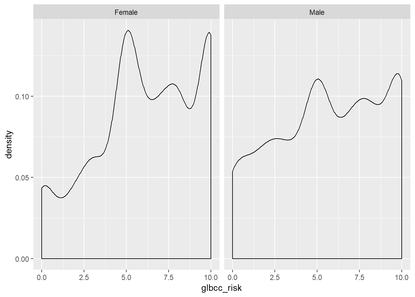.png?revision=1)
Based on the density plots, it appears that some differences exist between males and females regarding perceived climate change risk. We can also use the by command to see the mean of climate change risk for males and females.
by(ds$glbcc_risk, ds$f.gend, mean, na.rm=TRUE)## ds$f.gend: Female
## [1] 6.134259
## --------------------------------------------------------
## ds$f.gend: Male
## [1] 5.670577Again there appears to be a difference, with females perceiving greater risk on average (6.13) than males (5.67). However, we want to know whether these differences are statistically significant. To test for the statistical significance of the difference between groups, we use a t-test.
5.4.1 t-tests
The t-test is based on the tt distribution. The tt distribution, also known as the Student’s tt distribution, is the probability distribution for sample estimates. It has similar properties and is related to, the normal distribution. The normal distribution is based on a population where μμ and σ2σ2 are known; however, the tt distribution is based on a sample where μμ and σ2σ2 are estimated, as the mean ¯XX¯ and variance s2xsx2. The mean of the tt distribution, like the normal distribution, is 00, but the variance, s2xsx2, is conditioned by n−1n−1 degrees of freedom(df). Degrees of freedom are the values used to calculate statistics that are “free” to vary.11 A tt distribution approaches the standard normal distribution as the number of degrees of freedom increases.
In summary, we want to know the difference of means between males and females, d=¯Xm−¯Xfd=X¯m−X¯f, and if that difference is statistically significant. This amounts to a hypothesis test where our working hypothesis, H1H1, is that males are less likely than females to view climate change as risky. The null hypothesis, HAHA, is that there is no difference between males and females regarding the risks associated with climate change. To test H1H1 we use the t-test, which is calculated:
t=¯Xm−¯XfSEd(5.6)(5.6)t=X¯m−X¯fSEd
Where SEdSEd is the of the estimated differences between the two groups. To estimate SEdSEd, we need the SE of the estimated mean for each group. The SE is calculated:
SE=s√n(5.7)(5.7)SE=sn
where ss is the s.d. of the variable. H1H1 states that there is a difference between males and females, therefore under H1H1 it is expected that t>0t>0 since zero is the mean of the tt distribution. However, under HAHA it is expected that t=0t=0.
We can calculate this in R. First, we calculate the nn size for males and females. Then we calculate the SE for males and females.
n.total <- length(ds$gender)
nM <- sum(ds$gender, na.rm=TRUE)
nF <- n.total-nM
by(ds$glbcc_risk, ds$f.gend, sd, na.rm=TRUE)
## ds$f.gend: Female
## [1] 2.981938
## --------------------------------------------------------
## ds$f.gend: Male
## [1] 3.180171sdM <- 2.82
seM <- 2.82/(sqrt(nM))
seM## [1] 0.08803907sdF <- 2.35
seF <- 2.35/(sqrt(nF))
seF## [1] 0.06025641Next, we need to calculate the SEdSEd:SEd=√SE2M+SE2F(5.8)(5.8)SEd=SEM2+SEF2
seD <- sqrt(seM^2+seF^2)
seD
## [1] 0.1066851Finally, we can calculate our t-score, and use the t.test function to check.
by(ds$glbcc_risk, ds$f.gend, mean, na.rm=TRUE)## ds$f.gend: Female
## [1] 6.134259
## --------------------------------------------------------
## ds$f.gend: Male
## [1] 5.670577meanF <- 6.96
meanM <- 6.42
t <- (meanF-meanM)/seD
t## [1] 5.061625t.test(ds$glbcc_risk~ds$gender)##
## Welch Two Sample t-test
##
## data: ds$glbcc_risk by ds$gender
## t = 3.6927, df = 2097.5, p-value = 0.0002275
## alternative hypothesis: true difference in means is not equal to 0
## 95 percent confidence interval:
## 0.2174340 0.7099311
## sample estimates:
## mean in group 0 mean in group 1
## 6.134259 5.670577For the difference in the perceived risk between women and men, we have a tt-value of 4.6. This result is greater than zero, as expected by H1H1. In addition, as shown in the t.test output the pp-value—the probability of obtaining our result if the population difference was 00—is extremely low at .0002275 (that’s the same as 2.275e-04). Therefore, we reject the null hypothesis and concluded that there are differences (on average) in the ways that males and females perceive climate change risk.
5.5 Summary
In this chapter we gained an understanding of inferential statistics, how to use them to place confidence intervals around an estimate, and an overview of how to use them to test hypotheses. In the next chapter, we turn, more formally, to testing hypotheses using crosstabs and by comparing means of different groups. We then continue to explore hypothesis testing and model building using regression analysis.
- It is important to keep in mind that, for purposes of theory building, the population of interest may not be finite. For example, if you theorize about the general properties of human behavior, many of the members of the human population are not yet (or are no longer) alive. Hence it is not possible to include all of the population of interest in your research. We, therefore, rely on samples.↩
- Of course, we also need to estimate changes – both gradual and abrupt – in how people behave over time, which is the province of time-series analysis.↩
- Wei Wang, David Rothschild, Sharad Goel, and Andrew Gelman (2014) ’’Forecasting Elections with Non-Representative Polls," Preprint submitted to International Journal of Forecasting March 31, 2014.↩
- In a difference of means test across two groups, we “use up” one observation when we separate the observations into two groups. Hence the denominator reflects the loss of that used up observation: n-1.↩