7.1: heoretical Models

Models, as discussed earlier, are an essential component in theory building. They simplify theoretical concepts, provide a precise way to evaluate relationships between variables, and serve as a vehicle for hypothesis testing. As discussed in Chapter 1, one of the central features of a theoretical model is the presumption of causality, and causality is based on three factors: time ordering (observational or theoretical), co-variation, and non-spuriousness. Of these three assumptions, co-variation is the one analyzed using OLS. The often-repeated adage, correlation is not causation’’ is key. Causation is driven by theory, but co-variation is a critical part of empirical hypothesis testing.

When describing relationships, it is important to distinguish between those that are deterministic versus stochastic. Deterministic relationships are “fully determined” such that, knowing the values of the independent variable, you can perfectly explain (or predict) the value of the dependent variable. Philosophers of Old (like Kant) imagined the universe to be like a massive and complex clock which, once wound up and set ticking, would permit perfect prediction of the future if you had all the information on the starting conditions. There is no “error” in the prediction. Stochastic relationships, on the other hand, include an irreducible random component, such that the independent variables permit only a partial prediction of the dependent variable. But that stochastic (or random) component of the variation in the dependent variable has a probability distribution that can be analyzed statistically.

7.1.1 Deterministic Linear Model

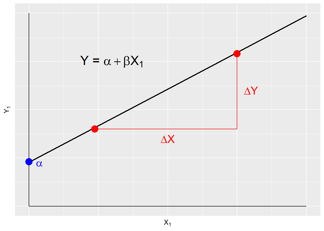
The deterministic linear model serves as the basis for evaluating theoretical models. It is expressed as:

Yi=α+βXi(7.1)(7.1)Yi=α+βXi

A deterministic model is systematic and contains no error, therefore YY is perfectly predicted by XX. This is illustrated in Figure \(\PageIndex{1}\). αα and ββ are the model parameters and are constant terms. ββ is the slope or the change in YY over the change in XX. αα is the intercept, or the value of YY when XX is zero.

Figure \(\PageIndex{1}\): Deterministic Model

Given that in social science we rarely work with deterministic models, nearly all models contain a stochastic, or random, component.

7.1.2 Stochastic Linear Model

The stochastic, or statistical, the linear model contains a systematic component, Y=α+βY=α+β, and a stochastic component called the error term. The error term is the difference between the expected value of YiYi and the observed value of YiYi; Yi−μYi−μ. This model is expressed as:

Yi=α+βXi+ϵi(7.2)(7.2)Yi=α+βXi+ϵi

where ϵiϵi is the error term. In the deterministic model, each value of YY fits along the regression line, however in a stochastic model, the expected value of YY is conditioned by the values of XX. This is illustrated in Figure \(\PageIndex{2}\).

Figure \(\PageIndex{2}\): Stochastic Linear Model

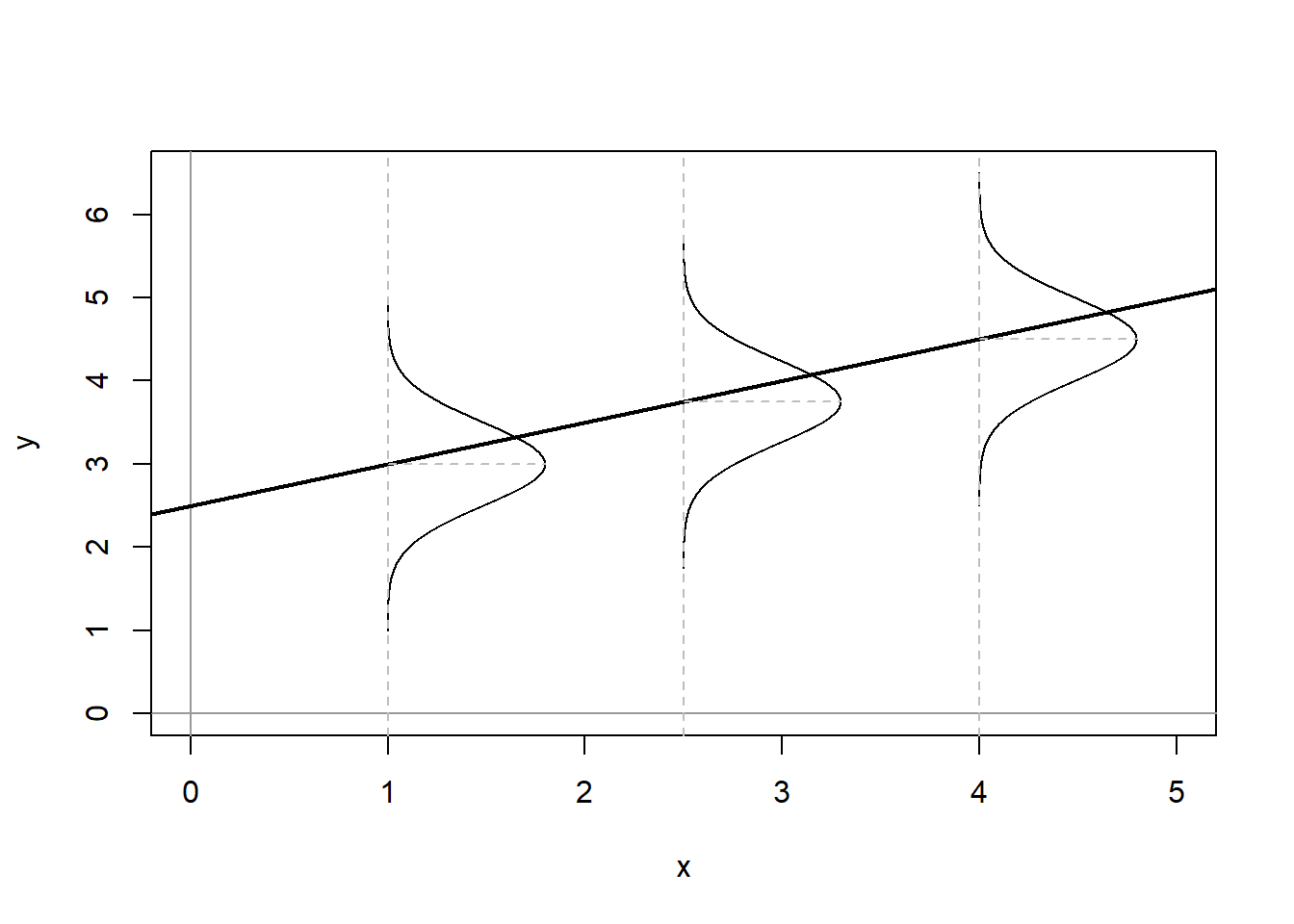
Figure \(\PageIndex{2}\) shows the conditional population distributions of YY for several values of X,p(Y|X)X,p(Y|X). The conditional means of YY given XX are denoted μμ.

μi≡E(Yi)≡E(Y|Xi)=α+βXi(7.3)(7.3)μi≡E(Yi)≡E(Y|Xi)=α+βXi

where - α=E(Y)≡μα=E(Y)≡μ when X=0X=0 - Each 1 unit increase in XX increases E(Y)E(Y) by ββ

However, in the stochastic linear model variation in YY is caused by more than XX, it is also caused by the error term ϵϵ. The error term is expressed as:

ϵi=Yi−E(Yi)=Yi−(α+βXi)=Yi−α−βXiϵi=Yi−E(Yi)=Yi−(α+βXi)=Yi−α−βXiTherefore;Yi=E(Yi)+ϵ=α+βXi+ϵiYi=E(Yi)+ϵ=α+βXi+ϵi

We make several important assumptions about the error term that are discussed in the next section.

7.1.3 Assumptions about the Error Term

There are three key assumptions about the error term; a) errors have identical distributions, b) errors are independent, and c) errors are normally distributed.¹⁴

Error Assumptions

• Errors have identical distributions

  E(ϵ2i)=σ2ϵE(ϵi2)=σϵ2

• Errors are independent of XX and other ϵiϵi

  E(ϵi)≡E(ϵ|xi)=0E(ϵi)≡E(ϵ|xi)=0

  and

  E(ϵi)≠E(ϵj)E(ϵi)≠E(ϵj) for i≠ji≠j

• Errors are normally distributed

  ϵi∼N(0,σ2ϵ)ϵi∼N(0,σϵ2)

Taken together these assumptions mean that the error term has a normal, independent, and identical distribution (normal i.i.d.). However, we don’t know if, in any particular case, these assumptions are met. Therefore we must estimate a linear model.