4.2: Finding Probabilities with the Normal Curve

Last updated
Save as PDF

Page ID: 7222

\( \newcommand{\vecs}[1]{\overset { \scriptstyle \rightharpoonup} {\mathbf{#1}} } \) \( \newcommand{\vecd}[1]{\overset{-\!-\!\rightharpoonup}{\vphantom{a}\smash {#1}}} \)\(\newcommand{\id}{\mathrm{id}}\) \( \newcommand{\Span}{\mathrm{span}}\) \( \newcommand{\kernel}{\mathrm{null}\,}\) \( \newcommand{\range}{\mathrm{range}\,}\) \( \newcommand{\RealPart}{\mathrm{Re}}\) \( \newcommand{\ImaginaryPart}{\mathrm{Im}}\) \( \newcommand{\Argument}{\mathrm{Arg}}\) \( \newcommand{\norm}[1]{\| #1 \|}\) \( \newcommand{\inner}[2]{\langle #1, #2 \rangle}\) \( \newcommand{\Span}{\mathrm{span}}\) \(\newcommand{\id}{\mathrm{id}}\) \( \newcommand{\Span}{\mathrm{span}}\) \( \newcommand{\kernel}{\mathrm{null}\,}\) \( \newcommand{\range}{\mathrm{range}\,}\) \( \newcommand{\RealPart}{\mathrm{Re}}\) \( \newcommand{\ImaginaryPart}{\mathrm{Im}}\) \( \newcommand{\Argument}{\mathrm{Arg}}\) \( \newcommand{\norm}[1]{\| #1 \|}\) \( \newcommand{\inner}[2]{\langle #1, #2 \rangle}\) \( \newcommand{\Span}{\mathrm{span}}\)\(\newcommand{\AA}{\unicode[.8,0]{x212B}}\)

If we want to find the probability of a score falling in a certain range, e.g., between 3 and 7, or more than 12, we can use the normal to determine that probability. Our ability to make that determination is based on some known characteristics on the normal curve. We know that for all normal curves 68.26% of all scores fall within one standard deviation of the mean, that 95.44% fall within two standard deviations, and that 99.72% fall within three standard deviations. (The normal distribution is dealt with more formally in the next chapter.) So, we know that something that is three or more standard deviations above the mean is pretty rare. Figure \(\PageIndex{1}\) illustrates the probabilities associated with the normal curve.⁷

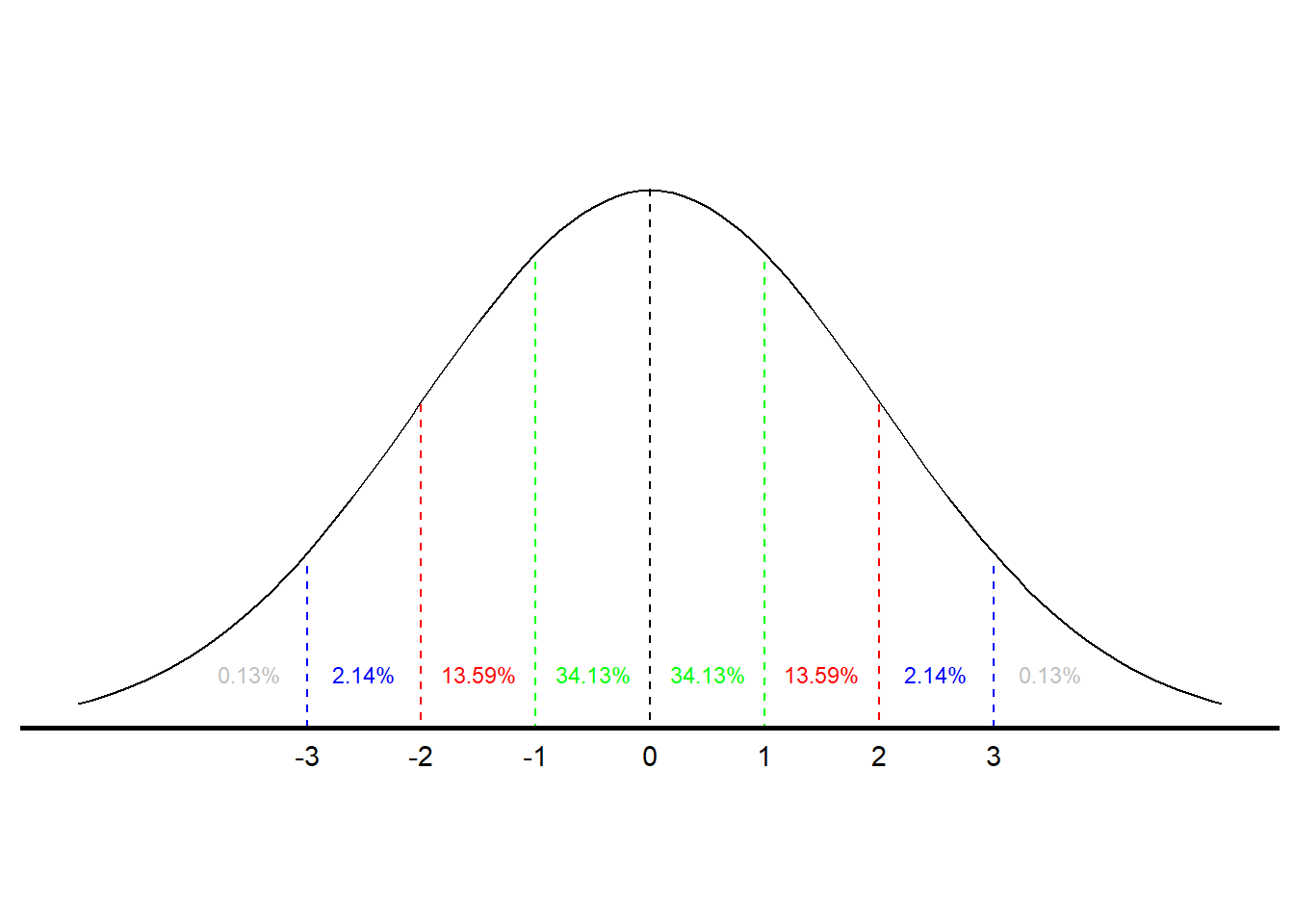
Figure \(\PageIndex{1}\): Area under the Normal Curve

According to Figure \(\PageIndex{1}\), there is a .3413 probability of an observation falling between the mean and one standard deviation above the mean and, therefore, a .6826 probability of a score falling within (+/−)(+/−) one standard deviation of the mean. There is also a .8413 probability of a score being one standard deviation above the mean or less (.5 probability of a score falling below the mean and a .3413 probability of a score falling between the mean and one standard deviation above it). (Using the language we learned in Chapter 3, another way to articulate that finding is to say that a score one standard deviation above the mean is at the 84th percentile.) There is also a .1587 probability of a score being a standard deviation above the mean or higher (1.0−.8413)(1.0−.8413).

Intelligence tests have a mean of 100 and a standard deviation of 15. Someone with an IQ of 130, then, is two standard deviations above the mean, meaning they score higher than 97.72% of the population. Suppose, though, your IQ is 140. Using Figure \(\PageIndex{1}\) would enable us only to approximate how high that score is. To find out more precisely, we have to find out how many standard deviations above the mean 140 is and then go to a more precise normal curve table.

To find out how many standard deviations from the mean an observation is, we calculated a standardized, or Z-score. The formula to convert a raw score to a Z-score is:

Z=x−μσ(4.4)(4.4)Z=x−μσ

In this case, the ZZ-score is 140−100/15140−100/15 or 2.672.67. Looking at the formula, you can see that a Z-score of zero puts that score at the mean; a ZZ-score of one is one standard deviation above the mean, and a ZZ-score of 2.672.67 is 2.672.67 standard deviations above the mean.

The next step is to go to a normal curve table to interpret that Z-score. Table @ref(fig: Normal_Curve) at the end of the chapter contains such a table. To use the table you combine rows and columns to find a score of 2.67. Where they cross we see the value .4962. That value means there is a .4962 probability of scoring between the mean and a ZZ-score of 2.67. Since there is a .5 probability of scoring below the mean adding the two values together gives a .9962 probability of finding an IQ of 140 or lower or a .0038 probability of someone having an IQ of 140 or better.

Bernoulli Probabilities

We can use a calculation known as the Bernoulli Process to determine the probability of a certain number of successes in a given number of trials. For example, if you want to know the probability of getting exactly three heads when you flip a coin four times, you can use the Bernoulli calculation. To perform the calculation you need to determine the number of trials (n)(n), the number of successes you care about (k)(k), the probability of success on a single trial (p)(p), and the probability (q)(q) of not a success (1−p(1−p or q)q). The operative formula is:

(n!k!(n−k)!)∗pk∗qn−k(n!k!(n−k)!)∗pk∗qn−k

The symbol n!n! is n factorial" or n∗(n−1)∗(n−2)n∗(n−1)∗(n−2) … ∗1∗1. So if you want to know the probability of getting three heads on four flips of a coin, n=4n=4, k=3k=3, p=.5p=.5, and q=.5q=.5:

(4!3!(4−3)!)∗.53∗.54−3=.25(4!3!(4−3)!)∗.53∗.54−3=.25

The Bernoulli process can be used only when both n∗pn∗p and n∗qn∗q are greater than ten. It is also most useful when you are interested in exactly kk successes. If you want to know the probability of kk or more, or kk or fewer successes, it is easier to use the normal curve. Bernoulli could still be used if your data is discrete, but you would have to do repeated calculations.