15.3: Multiple Linear Regression

The simple linear regression model that we’ve discussed up to this point assumes that there’s a single predictor variable that you’re interested in, in this case dan.sleep. In fact, up to this point, every statistical tool that we’ve talked about has assumed that your analysis uses one predictor variable and one outcome variable. However, in many (perhaps most) research projects you actually have multiple predictors that you want to examine. If so, it would be nice to be able to extend the linear regression framework to be able to include multiple predictors. Perhaps some kind of multiple regression model would be in order?

Multiple regression is conceptually very simple. All we do is add more terms to our regression equation. Let’s suppose that we’ve got two variables that we’re interested in; perhaps we want to use both dan.sleep and baby.sleep to predict the dan.grump variable. As before, we let Y_i refer to my grumpiness on the i-th day. But now we have two X variables: the first corresponding to the amount of sleep I got and the second corresponding to the amount of sleep my son got. So we’ll let X_i1 refer to the hours I slept on the i-th day, and X_i2 refers to the hours that the baby slept on that day. If so, then we can write our regression model like this:

Y_i = b₂ X_i2 + b₁ X_i1 + b₀ + ϵ_i

As before, ϵi is the residual associated with the i-th observation, \(\ \epsilon_i = Y_i - \hat{Y_i}\). In this model, we now have three coefficients that need to be estimated: b₀ is the intercept, b₁ is the coefficient associated with my sleep, and b₂ is the coefficient associated with my son’s sleep. However, although the number of coefficients that need to be estimated has changed, the basic idea of how the estimation works is unchanged: our estimated coefficients \(\ \hat{b_0}\), \(\ \hat{b_1}\) and \(\ \hat{b_2}\) are those that minimise the sum squared residuals.

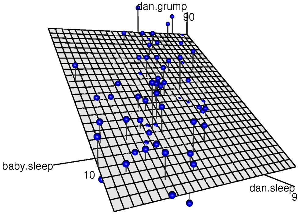
Figure 15.6: A 3D visualisation of a multiple regression model. There are two predictors in the model, dan.sleep and baby.sleep; the outcome variable is dan.grump. Together, these three variables form a 3D space: each observation (blue dots) is a point in this space. In much the same way that a simple linear regression model forms a line in 2D space, this multiple regression model forms a plane in 3D space. When we estimate the regression coefficients, what we’re trying to do is find a plane that is as close to all the blue dots as possible.

Doing it in R

Multiple regression in R is no different to simple regression: all we have to do is specify a more complicated formula when using the lm() function. For example, if we want to use both dan.sleep and baby.sleep as predictors in our attempt to explain why I’m so grumpy, then the formula we need is this:

   dan.grump ~ dan.sleep + baby.sleep

Notice that, just like last time, I haven’t explicitly included any reference to the intercept term in this formula; only the two predictor variables and the outcome. By default, the lm() function assumes that the model should include an intercept (though you can get rid of it if you want). In any case, I can create a new regression model – which I’ll call regression.2 – using the following command:

regression.2 <- lm( formula = dan.grump ~ dan.sleep + baby.sleep,  
                     data = parenthood )

And just like last time, if we print() out this regression model we can see what the estimated regression coefficients are:

print( regression.2 )

## 
## Call:
## lm(formula = dan.grump ~ dan.sleep + baby.sleep, data = parenthood)
## 
## Coefficients:
## (Intercept)    dan.sleep   baby.sleep  
##   125.96557     -8.95025      0.01052

The coefficient associated with dan.sleep is quite large, suggesting that every hour of sleep I lose makes me a lot grumpier. However, the coefficient for baby.sleep is very small, suggesting that it doesn’t really matter how much sleep my son gets; not really. What matters as far as my grumpiness goes is how much sleep I get. To get a sense of what this multiple regression model looks like, Figure 15.6 shows a 3D plot that plots all three variables, along with the regression model itself.

Formula for the general case

The equation that I gave above shows you what a multiple regression model looks like when you include two predictors. Not surprisingly, then, if you want more than two predictors all you have to do is add more X terms and more b coefficients. In other words, if you have K predictor variables in the model then the regression equation looks like this:

\(Y_{i}=\left(\sum_{k=1}^{K} b_{k} X_{i k}\right)+b_{0}+\epsilon_{i}\)