13.5: The Paired-samples t-test

Regardless of whether we’re talking about the Student test or the Welch test, an independent samples t-test is intended to be used in a situation where you have two samples that are, well, independent of one another. This situation arises naturally when participants are assigned randomly to one of two experimental conditions, but it provides a very poor approximation to other sorts of research designs. In particular, a repeated measures design – in which each participant is measured (with respect to the same outcome variable) in both experimental conditions – is not suited for analysis using independent samples t-tests. For example, we might be interested in whether listening to music reduces people’s working memory capacity. To that end, we could measure each person’s working memory capacity in two conditions: with music, and without music. In an experimental design such as this one,¹⁹⁴ each participant appears in both groups. This requires us to approach the problem in a different way; by using the paired samples t-test.

data

The data set that we’ll use this time comes from Dr Chico’s class.¹⁹⁵ In her class, students take two major tests, one early in the semester and one later in the semester. To hear her tell it, she runs a very hard class, one that most students find very challenging; but she argues that by setting hard assessments, students are encouraged to work harder. Her theory is that the first test is a bit of a “wake up call” for students: when they realise how hard her class really is, they’ll work harder for the second test and get a better mark. Is she right? To test this, let’s have a look at the chico.Rdata file:

load( "./rbook-master/data/chico.Rdata" )
str(chico)

## 'data.frame':    20 obs. of  3 variables:
##  $ id         : Factor w/ 20 levels "student1","student10",..: 1 12 14 15 16 17 18 19 20 2 ...
##  $ grade_test1: num  42.9 51.8 71.7 51.6 63.5 58 59.8 50.8 62.5 61.9 ...
##  $ grade_test2: num  44.6 54 72.3 53.4 63.8 59.3 60.8 51.6 64.3 63.2 ...

The data frame chico contains three variables: an id variable that identifies each student in the class, the grade_test1 variable that records the student grade for the first test, and the grade_test2 variable that has the grades for the second test. Here’s the first six students:

head( chico )

##         id grade_test1 grade_test2
## 1 student1        42.9        44.6
## 2 student2        51.8        54.0
## 3 student3        71.7        72.3
## 4 student4        51.6        53.4
## 5 student5        63.5        63.8
## 6 student6        58.0        59.3

At a glance, it does seem like the class is a hard one (most grades are between 50% and 60%), but it does look like there’s an improvement from the first test to the second one. If we take a quick look at the descriptive statistics

library( psych )
describe( chico )

##             vars  n  mean   sd median trimmed  mad  min  max range  skew
## id*            1 20 10.50 5.92   10.5   10.50 7.41  1.0 20.0  19.0  0.00
## grade_test1    2 20 56.98 6.62   57.7   56.92 7.71 42.9 71.7  28.8  0.05
## grade_test2    3 20 58.38 6.41   59.7   58.35 6.45 44.6 72.3  27.7 -0.05
##             kurtosis   se
## id*            -1.38 1.32
## grade_test1    -0.35 1.48
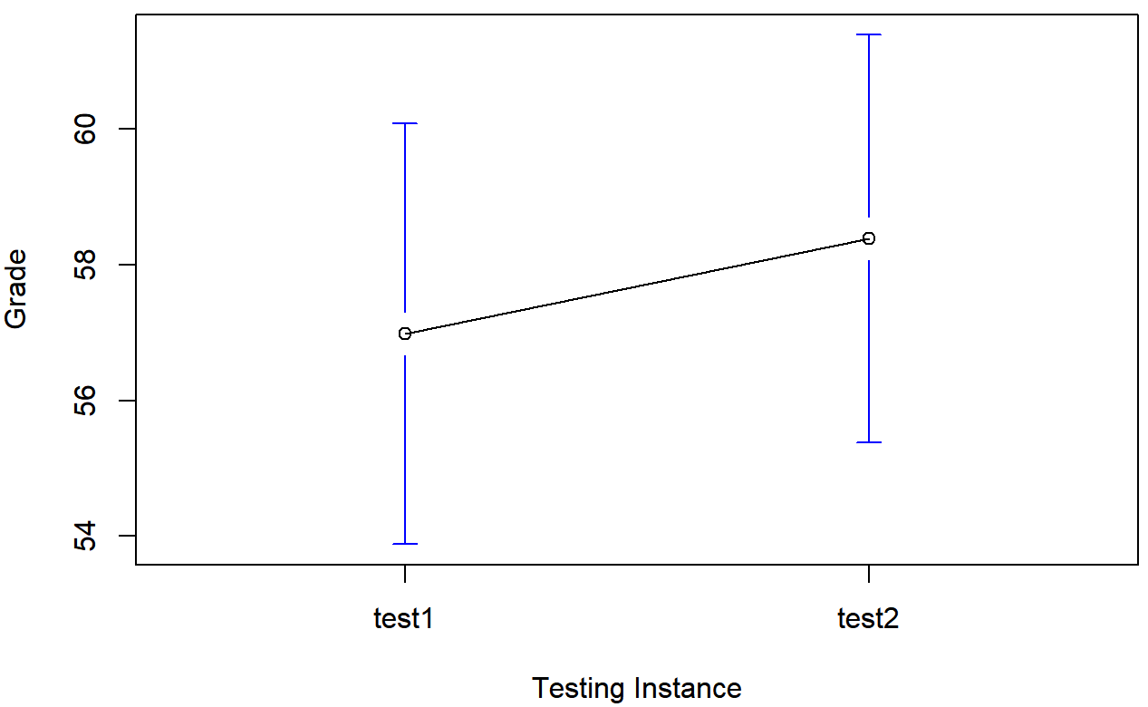
## grade_test2    -0.39 1.43

we see that this impression seems to be supported. Across all 20 students¹⁹⁶ the mean grade for the first test is 57%, but this rises to 58% for the second test. Although, given that the standard deviations are 6.6% and 6.4% respectively, it’s starting to feel like maybe the improvement is just illusory; maybe just random variation. This impression is reinforced when you see the means and confidence intervals plotted in Figure 13.11. If we were to rely on this plot alone, we’d come to the same conclusion that we got from looking at the descriptive statistics that the describe() function produced. Looking at how wide those confidence intervals are, we’d be tempted to think that the apparent improvement in student performance is pure chance.

Figure 13.11: Mean grade for test 1 and test 2, with associated 95% confidence intervals

Nevertheless, this impression is wrong. To see why, take a look at the scatterplot of the grades for test 1 against the grades for test 2. shown in Figure 13.12.

Figure 13.12: Scatterplot showing the individual grades for test 1 and test 2

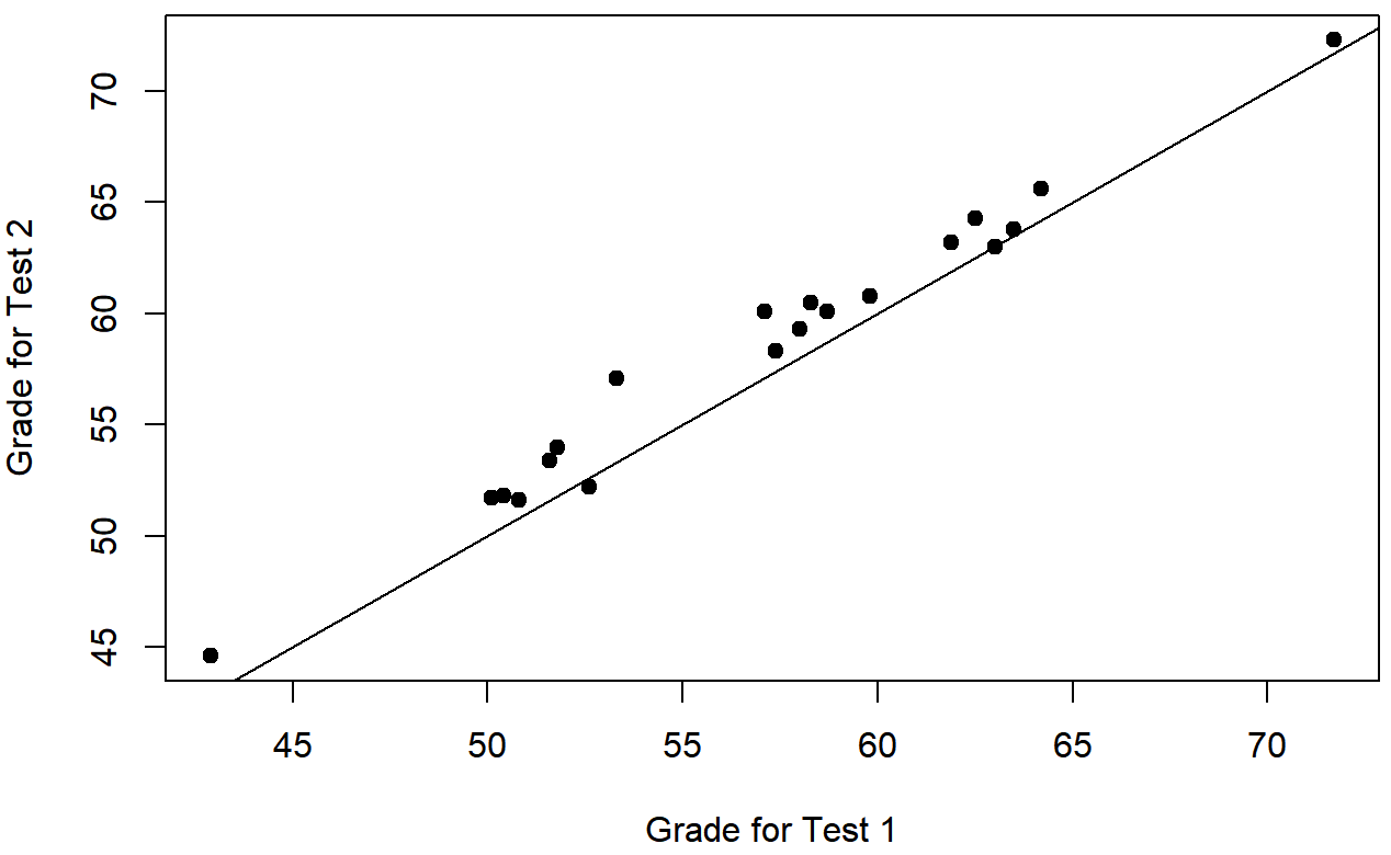
In this plot, each dot corresponds to the two grades for a given student: if their grade for test 1 (x co-ordinate) equals their grade for test 2 (y co-ordinate), then the dot falls on the line. Points falling above the line are the students that performed better on the second test. Critically, almost all of the data points fall above the diagonal line: almost all of the students do seem to have improved their grade, if only by a small amount. This suggests that we should be looking at the improvement made by each student from one test to the next, and treating that as our raw data. To do this, we’ll need to create a new variable for the improvement that each student makes, and add it to the chico data frame. The easiest way to do this is as follows:

chico$improvement <- chico$grade_test2 - chico$grade_test1 

Notice that I assigned the output to a variable called chico$improvement. That has the effect of creating a new variable called improvement inside the chico data frame. So now when I look at the chico data frame, I get an output that looks like this:

head( chico )

##         id grade_test1 grade_test2 improvement
## 1 student1        42.9        44.6         1.7
## 2 student2        51.8        54.0         2.2
## 3 student3        71.7        72.3         0.6
## 4 student4        51.6        53.4         1.8
## 5 student5        63.5        63.8         0.3
## 6 student6        58.0        59.3         1.3

Now that we’ve created and stored this improvement variable, we can draw a histogram showing the distribution of these improvement scores (using the hist() function), shown in Figure 13.13.

Figure 13.13: Histogram showing the improvement made by each student in Dr Chico’s class. Notice that almost the entire distribution is above zero: the vast majority of students did improve their performance from the first test to the second one

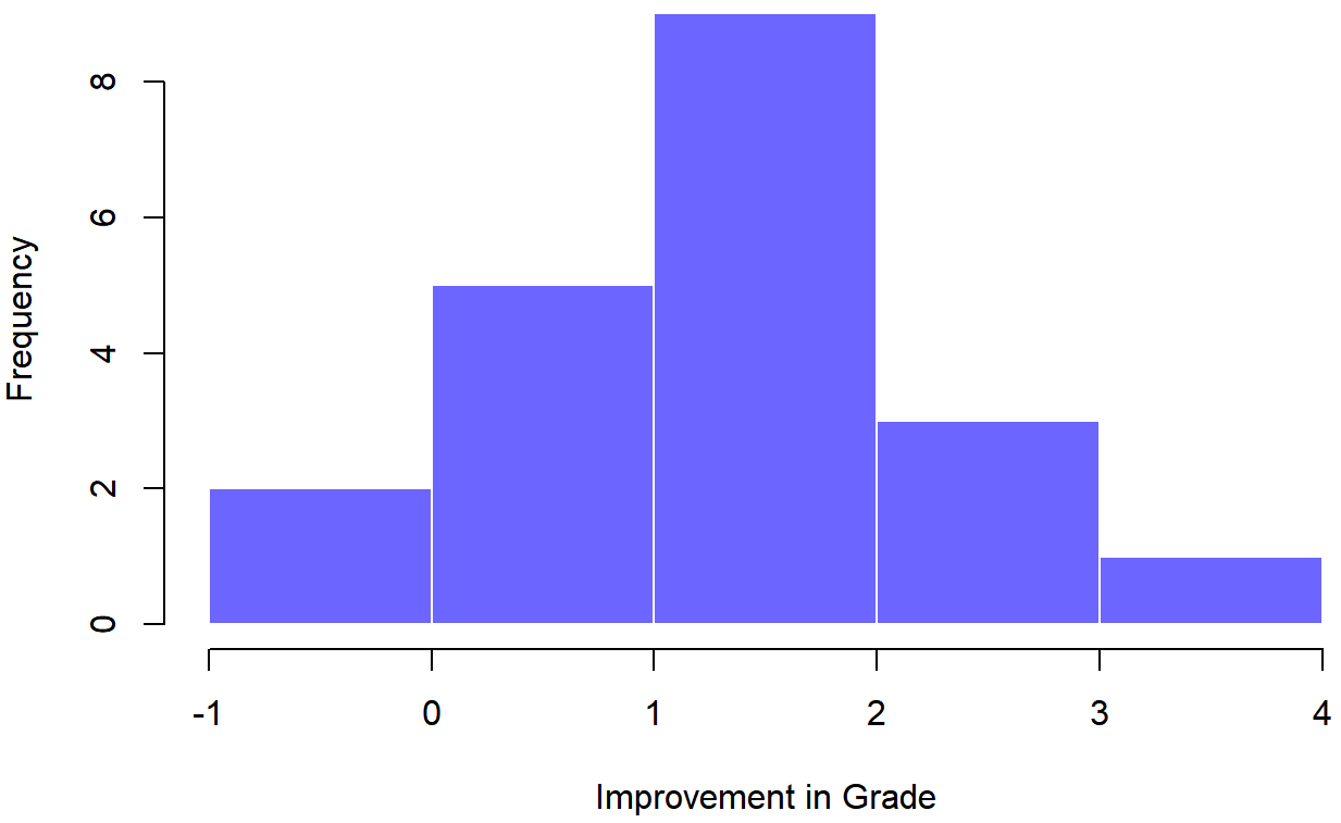
When we look at histogram, it’s very clear that there is a real improvement here. The vast majority of the students scored higher on the test 2 than on test 1, reflected in the fact that almost the entire histogram is above zero. In fact, if we use ciMean() to compute a confidence interval for the population mean of this new variable,

ciMean( x = chico$improvement )

##           2.5%    97.5%
## [1,] 0.9508686 1.859131

we see that it is 95% certain that the true (population-wide) average improvement would lie between 0.95% and 1.86%. So you can see, qualitatively, what’s going on: there is a real “within student” improvement (everyone improves by about 1%), but it is very small when set against the quite large “between student” differences (student grades vary by about 20% or so).

What is the paired samples t-test?

In light of the previous exploration, let’s think about how to construct an appropriate t test. One possibility would be to try to run an independent samples t-test using grade_test1 and grade_test2 as the variables of interest. However, this is clearly the wrong thing to do: the independent samples t-test assumes that there is no particular relationship between the two samples. Yet clearly that’s not true in this case, because of the repeated measures structure to the data. To use the language that I introduced in the last section, if we were to try to do an independent samples t-test, we would be conflating the within subject differences (which is what we’re interested in testing) with the between subject variability (which we are not).

The solution to the problem is obvious, I hope, since we already did all the hard work in the previous section. Instead of running an independent samples t-test on grade_test1 and grade_test2, we run a one-sample t-test on the within-subject difference variable, improvement. To formalise this slightly, if X_i1 is the score that the i-th participant obtained on the first variable, and X_i2 is the score that the same person obtained on the second one, then the difference score is:

D_i=X_i1−X_i2

Notice that the difference scores is variable 1 minus variable 2 and not the other way around, so if we want improvement to correspond to a positive valued difference, we actually want “test 2” to be our “variable 1”. Equally, we would say that μ_D=μ₁−μ₂ is the population mean for this difference variable. So, to convert this to a hypothesis test, our null hypothesis is that this mean difference is zero; the alternative hypothesis is that it is not:

H₀:μ_D=0

H₁:μ_D≠0

(this is assuming we’re talking about a two-sided test here). This is more or less identical to the way we described the hypotheses for the one-sample t-test: the only difference is that the specific value that the null hypothesis predicts is 0. And so our t-statistic is defined in more or less the same way too. If we let \(\ \bar{D}\) denote the mean of the difference scores, then

\(t=\dfrac{\bar{D}}{\operatorname{SE}(\bar{D})}\)

which is

\(t=\dfrac{\bar{D}}{\hat{\sigma}_{D} / \sqrt{N}}\)

where \(\ \hat{\sigma_D}\) is the standard deviation of the difference scores. Since this is just an ordinary, one-sample t-test, with nothing special about it, the degrees of freedom are still N−1. And that’s it: the paired samples t-test really isn’t a new test at all: it’s a one-sample t-test, but applied to the difference between two variables. It’s actually very simple; the only reason it merits a discussion as long as the one we’ve just gone through is that you need to be able to recognise when a paired samples test is appropriate, and to understand why it’s better than an independent samples t test.

Doing the test in R, part 1

How do you do a paired samples t-test in R. One possibility is to follow the process I outlined above: create a “difference” variable and then run a one sample t-test on that. Since we’ve already created a variable called chico$improvement, let’s do that:

oneSampleTTest( chico$improvement, mu=0 )

## 
##    One sample t-test 
## 
## Data variable:   chico$improvement 
## 
## Descriptive statistics: 
##             improvement
##    mean           1.405
##    std dev.       0.970
## 
## Hypotheses: 
##    null:        population mean equals 0 
##    alternative: population mean not equal to 0 
## 
## Test results: 
##    t-statistic:  6.475 
##    degrees of freedom:  19 
##    p-value:  <.001 
## 
## Other information: 
##    two-sided 95% confidence interval:  [0.951, 1.859] 
##    estimated effect size (Cohen's d):  1.448

The output here is (obviously) formatted exactly the same was as it was the last time we used the oneSampleTTest() function (Section 13.2), and it confirms our intuition. There’s an average improvement of 1.4% from test 1 to test 2, and this is significantly different from 0 (t(19)=6.48, p<.001).

However, suppose you’re lazy and you don’t want to go to all the effort of creating a new variable. Or perhaps you just want to keep the difference between one-sample and paired-samples tests clear in your head. If so, you can use the pairedSamplesTTest() function, also in the lsr package. Let’s assume that your data organised like they are in the chico data frame, where there are two separate variables, one for each measurement. The way to run the test is to input a one-sided formula, just like you did when running a test of association using the associationTest() function in Chapter 12. For the chico data frame, the formula that you need would be ~ grade_time2 + grade_time1. As usual, you’ll also need to input the name of the data frame too. So the command just looks like this:

pairedSamplesTTest( 
     formula = ~ grade_test2 + grade_test1, # one-sided formula listing the two variables
     data = chico                           # data frame containing the two variables 
  )

## 
##    Paired samples t-test 
## 
## Variables:  grade_test2 , grade_test1 
## 
## Descriptive statistics: 
##             grade_test2 grade_test1 difference
##    mean          58.385      56.980      1.405
##    std dev.       6.406       6.616      0.970
## 
## Hypotheses: 
##    null:        population means equal for both measurements
##    alternative: different population means for each measurement
## 
## Test results: 
##    t-statistic:  6.475 
##    degrees of freedom:  19 
##    p-value:  <.001 
## 
## Other information: 
##    two-sided 95% confidence interval:  [0.951, 1.859] 
##    estimated effect size (Cohen's d):  1.448

The numbers are identical to those that come from the one sample test, which of course they have to be given that the paired samples t-test is just a one sample test under the hood. However, the output is a bit more detailed:

This time around the descriptive statistics block shows you the means and standard deviations for the original variables, as well as for the difference variable (notice that it always defines the difference as the first listed variable mines the second listed one). The null hypothesis and the alternative hypothesis are now framed in terms of the original variables rather than the difference score, but you should keep in mind that in a paired samples test it’s still the difference score being tested. The statistical information at the bottom about the test result is of course the same as before.

Doing the test in R, part 2

The paired samples t-test is a little different from the other t-tests, because it is used in repeated measures designs. For the chico data, every student is “measured” twice, once for the first test, and again for the second test. Back in Section 7.7 I talked about the fact that repeated measures data can be expressed in two standard ways, known as wide form and long form. The chico data frame is in wide form: every row corresponds to a unique person. I’ve shown you the data in that form first because that’s the form that you’re most used to seeing, and it’s also the format that you’re most likely to receive data in. However, the majority of tools in R for dealing with repeated measures data expect to receive data in long form. The paired samples t-test is a bit of an exception that way.

As you make the transition from a novice user to an advanced one, you’re going to have to get comfortable with long form data, and switching between the two forms. To that end, I want to show you how to apply the pairedSamplesTTest() function to long form data. First, let’s use the wideToLong() function to create a long form version of the chico data frame. If you’ve forgotten how the wideToLong() function works, it might be worth your while quickly re-reading Section 7.7. Assuming that you’ve done so, or that you’re already comfortable with data reshaping, I’ll use it to create a new data frame called chico2:

chico2 <- wideToLong( chico, within="time" )
head( chico2 )

##         id improvement  time grade
## 1 student1         1.7 test1  42.9
## 2 student2         2.2 test1  51.8
## 3 student3         0.6 test1  71.7
## 4 student4         1.8 test1  51.6
## 5 student5         0.3 test1  63.5
## 6 student6         1.3 test1  58.0

As you can see, this has created a new data frame containing three variables: an id variable indicating which person provided the data, a time variable indicating which test the data refers to (i.e., test 1 or test 2), and a grade variable that records what score the person got on that test. Notice that this data frame is in long form: every row corresponds to a unique measurement. Because every person provides two observations (test 1 and test 2), there are two rows for every person. To see this a little more clearly, I’ll use the sortFrame() function to sort the rows of chico2 by id variable (see Section 7.6.3).

chico2 <- sortFrame( chico2, id )
head( chico2 )

##           id improvement  time grade
## 1   student1         1.7 test1  42.9
## 21  student1         1.7 test2  44.6
## 10 student10         1.3 test1  61.9
## 30 student10         1.3 test2  63.2
## 11 student11         1.4 test1  50.4
## 31 student11         1.4 test2  51.8

As you can see, there are two rows for “student1”: one showing their grade on the first test, the other showing their grade on the second test.¹⁹⁷

Okay, suppose that we were given the chico2 data frame to analyse. How would we run our paired samples t-test now? One possibility would be to use the longToWide() function (Section 7.7) to force the data back into wide form, and do the same thing that we did previously. But that’s sort of defeating the point, and besides, there’s an easier way. Let’s think about what how the chico2 data frame is structured: there are three variables here, and they all matter. The outcome measure is stored as the grade, and we effectively have two “groups” of measurements (test 1 and test 2) that are defined by the time points at which a test is given. Finally, because we want to keep track of which measurements should be paired together, we need to know which student obtained each grade, which is what the id variable gives us. So, when your data are presented to you in long form, we would want specify a two-sided formula and a data frame, in the same way that we do for an independent samples t-test: the formula specifies the outcome variable and the groups, so in this case it would be grade ~ time, and the data frame is chico2. However, we also need to tell it the id variable, which in this case is boringly called id. So our command is:

pairedSamplesTTest( 
     formula = grade ~ time,  # two sided formula: outcome ~ group
     data = chico2,           # data frame
     id = "id"                # name of the id variable
  )

## 
##    Paired samples t-test 
## 
## Outcome variable:   grade 
## Grouping variable:  time 
## ID variable:        id 
## 
## Descriptive statistics: 
##              test1  test2 difference
##    mean     56.980 58.385     -1.405
##    std dev.  6.616  6.406      0.970
## 
## Hypotheses: 
##    null:        population means equal for both measurements
##    alternative: different population means for each measurement
## 
## Test results: 
##    t-statistic:  -6.475 
##    degrees of freedom:  19 
##    p-value:  <.001 
## 
## Other information: 
##    two-sided 95% confidence interval:  [-1.859, -0.951] 
##    estimated effect size (Cohen's d):  1.448

Note that the name of the id variable is "id" and not id. Note that the id variable must be a factor. As of the current writing, you do need to include the quote marks, because the pairedSamplesTTest() function is expecting a character string that specifies the name of a variable. If I ever find the time I’ll try to relax this constraint.

As you can see, it’s a bit more detailed than the output from oneSampleTTest(). It gives you the descriptive statistics for the original variables, states the null hypothesis in a fashion that is a bit more appropriate for a repeated measures design, and then reports all the nuts and bolts from the hypothesis test itself. Not surprisingly the numbers the same as the ones that we saw last time.

One final comment about the pairedSamplesTTest() function. One of the reasons I designed it to be able handle long form and wide form data is that I want you to be get comfortable thinking about repeated measures data in both formats, and also to become familiar with the different ways in which R functions tend to specify models and tests for repeated measures data. With that last point in mind, I want to highlight a slightly different way of thinking about what the paired samples t-test is doing. There’s a sense in which what you’re really trying to do is look at how the outcome variable (grade) is related to the grouping variable (time), after taking account of the fact that there are individual differences between people (id). So there’s a sense in which id is actually a second predictor: you’re trying to predict the grade on the basis of the time and the id. With that in mind, the pairedSamplesTTest() function lets you specify a formula like this one

grade ~ time + (id)

This formula tells R everything it needs to know: the variable on the left (grade) is the outcome variable, the bracketed term on the right (id) is the id variable, and the other term on the right is the grouping variable (time). If you specify your formula that way, then you only need to specify the formula and the data frame, and so you can get away with using a command as simple as this one:

pairedSamplesTTest( 
     formula = grade ~ time + (id),
     data = chico2
  )

or you can drop the argument names and just do this:

> pairedSamplesTTest( grade ~ time + (id), chico2 )

These commands will produce the same output as the last one, I personally find this format a lot more elegant. That being said, the main reason for allowing you to write your formulas that way is that they’re quite similar to the way that mixed models (fancy pants repeated measures analyses) are specified in the lme4 package. This book doesn’t talk about mixed models (yet!), but if you go on to learn more statistics you’ll find them pretty hard to avoid, so I’ve tried to lay a little bit of the groundwork here.