10.5: Estimating a Confidence Interval

Statistics means never having to say you’re certain – Unknown origin¹⁵⁴ but I’ve never found the original source.

Up to this point in this chapter, I’ve outlined the basics of sampling theory which statisticians rely on to make guesses about population parameters on the basis of a sample of data. As this discussion illustrates, one of the reasons we need all this sampling theory is that every data set leaves us with a some of uncertainty, so our estimates are never going to be perfectly accurate. The thing that has been missing from this discussion is an attempt to quantify the amount of uncertainty that attaches to our estimate. It’s not enough to be able guess that, say, the mean IQ of undergraduate psychology students is 115 (yes, I just made that number up). We also want to be able to say something that expresses the degree of certainty that we have in our guess. For example, it would be nice to be able to say that there is a 95% chance that the true mean lies between 109 and 121. The name for this is a confidence interval for the mean.

Armed with an understanding of sampling distributions, constructing a confidence interval for the mean is actually pretty easy. Here’s how it works. Suppose the true population mean is μ and the standard deviation is σ. I’ve just finished running my study that has N participants, and the mean IQ among those participants is \(\bar{X}\). We know from our discussion of the central limit theorem (Section 10.3.3 that the sampling distribution of the mean is approximately normal. We also know from our discussion of the normal distribution Section 9.5 that there is a 95% chance that a normally-distributed quantity will fall within two standard deviations of the true mean. To be more precise, we can use the qnorm() function to compute the 2.5th and 97.5th percentiles of the normal distribution

qnorm( p = c(.025, .975) )

## [1] -1.959964  1.959964

Okay, so I lied earlier on. The more correct answer is that 95% chance that a normally-distributed quantity will fall within 1.96 standard deviations of the true mean. Next, recall that the standard deviation of the sampling distribution is referred to as the standard error, and the standard error of the mean is written as SEM. When we put all these pieces together, we learn that there is a 95% probability that the sample mean \(\bar{X}\) that we have actually observed lies within 1.96 standard errors of the population mean. Mathematically, we write this as:

μ−(1.96×SEM) ≤ \(\bar{X}\) ≤ μ+(1.96×SEM)

where the SEM is equal to σ/\(\sqrt{N}\), and we can be 95% confident that this is true. However, that’s not answering the question that we’re actually interested in. The equation above tells us what we should expect about the sample mean, given that we know what the population parameters are. What we want is to have this work the other way around: we want to know what we should believe about the population parameters, given that we have observed a particular sample. However, it’s not too difficult to do this. Using a little high school algebra, a sneaky way to rewrite our equation is like this:

\(\bar{X}\)−(1.96×SEM) ≤ μ ≤ \(\bar{X}\)+(1.96×SEM)

What this is telling is is that the range of values has a 95% probability of containing the population mean μ. We refer to this range as a 95% confidence interval, denoted CI₉₅. In short, as long as N is sufficiently large – large enough for us to believe that the sampling distribution of the mean is normal – then we can write this as our formula for the 95% confidence interval:

\(\mathrm{CI}_{95}=\bar{X} \pm\left(1.96 \times \dfrac{\sigma}{\sqrt{N}}\right)\)

Of course, there’s nothing special about the number 1.96: it just happens to be the multiplier you need to use if you want a 95% confidence interval. If I’d wanted a 70% confidence interval, I could have used the qnorm() function to calculate the 15th and 85th quantiles:

qnorm( p = c(.15, .85) )

## [1] -1.036433  1.036433

and so the formula for CI₇₀ would be the same as the formula for CI₉₅ except that we’d use 1.04 as our magic number rather than 1.96.

slight mistake in the formula

As usual, I lied. The formula that I’ve given above for the 95% confidence interval is approximately correct, but I glossed over an important detail in the discussion. Notice my formula requires you to use the standard error of the mean, SEM, which in turn requires you to use the true population standard deviation σ. Yet, in Section @ref(pointestimates I stressed the fact that we don’t actually know the true population parameters. Because we don’t know the true value of σ, we have to use an estimate of the population standard deviation \(\hat{σ}\) instead. This is pretty straightforward to do, but this has the consequence that we need to use the quantiles of the t-distribution rather than the normal distribution to calculate our magic number; and the answer depends on the sample size. When N is very large, we get pretty much the same value using qt() that we would if we used qnorm()…

N <- 10000   # suppose our sample size is 10,000
qt( p = .975, df = N-1)   # calculate the 97.5th quantile of the t-dist

## [1] 1.960201

But when N is small, we get a much bigger number when we use the t distribution:

N <- 10   # suppose our sample size is 10
qt( p = .975, df = N-1)   # calculate the 97.5th quantile of the t-dist

## [1] 2.262157

There’s nothing too mysterious about what’s happening here. Bigger values mean that the confidence interval is wider, indicating that we’re more uncertain about what the true value of μ actually is. When we use the t distribution instead of the normal distribution, we get bigger numbers, indicating that we have more uncertainty. And why do we have that extra uncertainty? Well, because our estimate of the population standard deviation ^σ might be wrong! If it’s wrong, it implies that we’re a bit less sure about what our sampling distribution of the mean actually looks like… and this uncertainty ends up getting reflected in a wider confidence interval.

Interpreting a confidence interval

The hardest thing about confidence intervals is understanding what they mean. Whenever people first encounter confidence intervals, the first instinct is almost always to say that “there is a 95% probabaility that the true mean lies inside the confidence interval”. It’s simple, and it seems to capture the common sense idea of what it means to say that I am “95% confident”. Unfortunately, it’s not quite right. The intuitive definition relies very heavily on your own personal beliefs about the value of the population mean. I say that I am 95% confident because those are my beliefs. In everyday life that’s perfectly okay, but if you remember back to Section 9.2, you’ll notice that talking about personal belief and confidence is a Bayesian idea. Personally (speaking as a Bayesian) I have no problem with the idea that the phrase “95% probability” is allowed to refer to a personal belief. However, confidence intervals are not Bayesian tools. Like everything else in this chapter, confidence intervals are frequentist tools, and if you are going to use frequentist methods then it’s not appropriate to attach a Bayesian interpretation to them. If you use frequentist methods, you must adopt frequentist interpretations!

Okay, so if that’s not the right answer, what is? Remember what we said about frequentist probability: the only way we are allowed to make “probability statements” is to talk about a sequence of events, and to count up the frequencies of different kinds of events. From that perspective, the interpretation of a 95% confidence interval must have something to do with replication. Specifically: if we replicated the experiment over and over again and computed a 95% confidence interval for each replication, then 95% of those intervals would contain the true mean. More generally, 95% of all confidence intervals constructed using this procedure should contain the true population mean. This idea is illustrated in Figure 10.13, which shows 50 confidence intervals constructed for a “measure 10 IQ scores” experiment (top panel) and another 50 confidence intervals for a “measure 25 IQ scores” experiment (bottom panel). A bit fortuitously, across the 100 replications that I simulated, it turned out that exactly 95 of them contained the true mean.

Figure 10.13: 95% confidence intervals. The top (panel a) shows 50 simulated replications of an experiment in which we measure the IQs of 10 people. The dot marks the location of the sample mean, and the line shows the 95% confidence interval. In total 47 of the 50 confidence intervals do contain the true mean (i.e., 100), but the three intervals marked with asterisks do not. The lower graph (panel b) shows a similar simulation, but this time we simulate replications of an experiment that measures the IQs of 25 people.

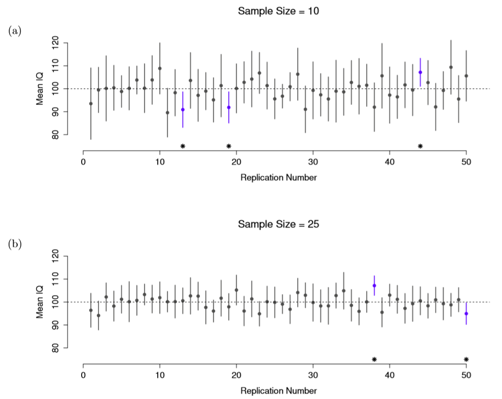
The critical difference here is that the Bayesian claim makes a probability statement about the population mean (i.e., it refers to our uncertainty about the population mean), which is not allowed under the frequentist interpretation of probability because you can’t “replicate” a population! In the frequentist claim, the population mean is fixed and no probabilistic claims can be made about it. Confidence intervals, however, are repeatable so we can replicate experiments. Therefore a frequentist is allowed to talk about the probability that the confidence interval (a random variable) contains the true mean; but is not allowed to talk about the probability that the true population mean (not a repeatable event) falls within the confidence interval.

I know that this seems a little pedantic, but it does matter. It matters because the difference in interpretation leads to a difference in the mathematics. There is a Bayesian alternative to confidence intervals, known as credible intervals. In most situations credible intervals are quite similar to confidence intervals, but in other cases they are drastically different. As promised, though, I’ll talk more about the Bayesian perspective in Chapter 17.

Calculating confidence intervals in R

As far as I can tell, the core packages in R don’t include a simple function for calculating confidence intervals for the mean. They do include a lot of complicated, extremely powerful functions that can be used to calculate confidence intervals associated with lots of different things, such as the confint() function that we’ll use in Chapter 15. But I figure that when you’re first learning statistics, it might be useful to start with something simpler. As a consequence, the lsr package includes a function called ciMean() which you can use to calculate your confidence intervals. There are two arguments that you might want to specify:¹⁵⁵

• x. This should be a numeric vector containing the data.
• conf. This should be a number, specifying the confidence level. By default, conf = .95, since 95% confidence intervals are the de facto standard in psychology.

So, for example, if I load the afl24.Rdata file, calculate the confidence interval associated with the mean attendance:

> ciMean( x = afl$attendance )
    2.5%    97.5% 
31597.32 32593.12 

Hopefully that’s fairly clear.

Plotting confidence intervals in R

There’s several different ways you can draw graphs that show confidence intervals as error bars. I’ll show three versions here, but this certainly doesn’t exhaust the possibilities. In doing so, what I’m assuming is that you want to draw is a plot showing the means and confidence intervals for one variable, broken down by different levels of a second variable. For instance, in our afl data that we discussed earlier, we might be interested in plotting the average attendance by year. I’ll do this using two different functions, bargraph.CI() and lineplot.CI() (both of which are in the sciplot package). Assuming that you’ve installed these packages on your system (see Section 4.2 if you’ve forgotten how to do this), you’ll need to load them. You’ll also need to load the lsr package, because we’ll make use of the ciMean() function to actually calculate the confidence intervals

load( "./rbook-master/data/afl24.Rdata" )  # contains the "afl" data frame
library( sciplot )     # bargraph.CI() and lineplot.CI() functions
library( lsr )         # ciMean() function

Here’s how to plot the means and confidence intervals drawn using bargraph.CI().

bargraph.CI( x.factor = year,            # grouping variable 
              response = attendance,      # outcome variable
              data = afl,                 # data frame with the variables
              ci.fun= ciMean,             # name of the function to calculate CIs
              xlab = "Year",              # x-axis label
              ylab = "Average Attendance" # y-axis label
 )

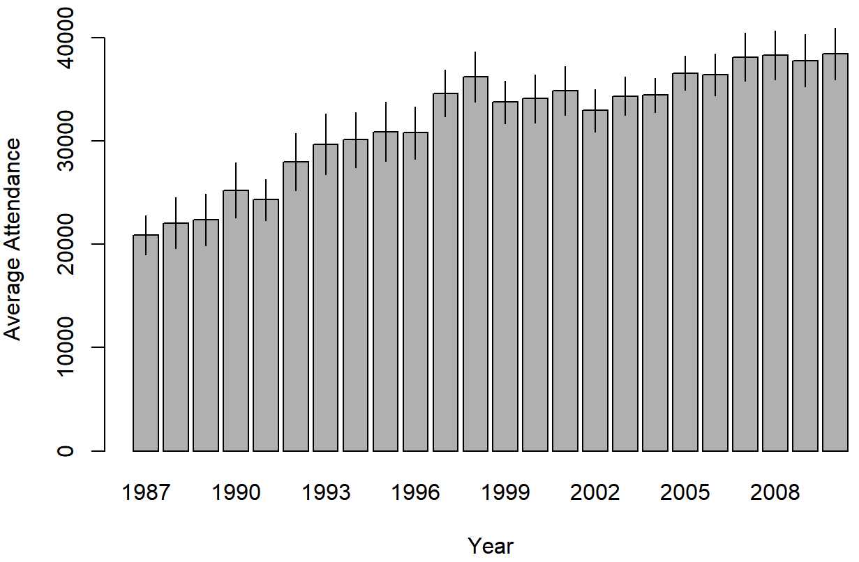
Figure 10.14: Means and 95% confidence intervals for AFL attendance, plotted separately for each year from 1987 to 2010. This graph was drawn using the bargraph.CI() function.

We can use the same arguments when calling the lineplot.CI() function:

lineplot.CI( x.factor = year,            # grouping variable 
             response = attendance,      # outcome variable
             data = afl,                 # data frame with the variables
             ci.fun= ciMean,             # name of the function to calculate CIs
             xlab = "Year",              # x-axis label
             ylab = "Average Attendance" # y-axis label
)

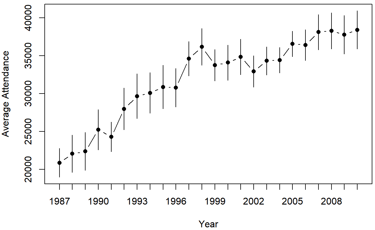
Figure 10.15: Means and 95% confidence intervals for AFL attendance, plotted separately for each year from 1987 to 2010. This graph was drawn using the lineplot.CI() function.