9.4: The Binomial Distribution

As you might imagine, probability distributions vary enormously, and there’s an enormous range of distributions out there. However, they aren’t all equally important. In fact, the vast majority of the content in this book relies on one of five distributions: the binomial distribution, the normal distribution, the t distribution, the χ² (“chi-square”) distribution and the F distribution. Given this, what I’ll do over the next few sections is provide a brief introduction to all five of these, paying special attention to the binomial and the normal. I’ll start with the binomial distribution, since it’s the simplest of the five.

Introducing the binomial

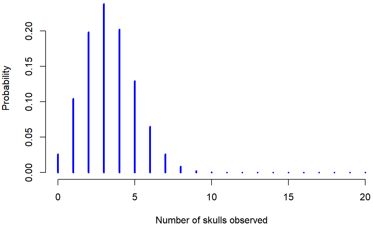
The theory of probability originated in the attempt to describe how games of chance work, so it seems fitting that our discussion of the binomial distribution should involve a discussion of rolling dice and flipping coins. Let’s imagine a simple “experiment”: in my hot little hand I’m holding 20 identical six-sided dice. On one face of each die there’s a picture of a skull; the other five faces are all blank. If I proceed to roll all 20 dice, what’s the probability that I’ll get exactly 4 skulls? Assuming that the dice are fair, we know that the chance of any one die coming up skulls is 1 in 6; to say this another way, the skull probability for a single die is approximately .167. This is enough information to answer our question, so let’s have a look at how it’s done.

As usual, we’ll want to introduce some names and some notation. We’ll let N denote the number of dice rolls in our experiment; which is often referred to as the size parameter of our binomial distribution. We’ll also use θ to refer to the the probability that a single die comes up skulls, a quantity that is usually called the success probability of the binomial.¹⁴³ Finally, we’ll use X to refer to the results of our experiment, namely the number of skulls I get when I roll the dice. Since the actual value of X is due to chance, we refer to it as a random variable. In any case, now that we have all this terminology and notation, we can use it to state the problem a little more precisely. The quantity that we want to calculate is the probability that X=4 given that we know that θ=.167 and N=20. The general “form” of the thing I’m interested in calculating could be written as

P(X | θ,N)

and we’re interested in the special case where X=4, θ=.167 and N=20. There’s only one more piece of notation I want to refer to before moving on to discuss the solution to the problem. If I want to say that X is generated randomly from a binomial distribution with parameters θ and N, the notation I would use is as follows:

X∼Binomial(θ,N)

Yeah, yeah. I know what you’re thinking: notation, notation, notation. Really, who cares? Very few readers of this book are here for the notation, so I should probably move on and talk about how to use the binomial distribution. I’ve included the formula for the binomial distribution in Table 9.2, since some readers may want to play with it themselves, but since most people probably don’t care that much and because we don’t need the formula in this book, I won’t talk about it in any detail. Instead, I just want to show you what the binomial distribution looks like. To that end, Figure 9.3 plots the binomial probabilities for all possible values of X for our dice rolling experiment, from X=0 (no skulls) all the way up to X=20 (all skulls). Note that this is basically a bar chart, and is no different to the “pants probability” plot I drew in Figure 9.2. On the horizontal axis we have all the possible events, and on the vertical axis we can read off the probability of each of those events. So, the probability of rolling 4 skulls out of 20 times is about 0.20 (the actual answer is 0.2022036, as we’ll see in a moment). In other words, you’d expect that to happen about 20% of the times you repeated this experiment.

Figure 9.3: The binomial distribution with size parameter of N=20 and an underlying success probability of theta=1/6. Each vertical bar depicts the probability of one specific outcome (i.e., one possible value of X). Because this is a probability distribution, each of the probabilities must be a number between 0 and 1, and the heights of the bars must sum to 1 as well.

Working with the binomial distribution in R

Although some people find it handy to know the formulas in Table 9.2, most people just want to know how to use the distributions without worrying too much about the maths. To that end, R has a function called dbinom() that calculates binomial probabilities for us. The main arguments to the function are

• x. This is a number, or vector of numbers, specifying the outcomes whose probability you’re trying to calculate.
• size. This is a number telling R the size of the experiment.
• prob. This is the success probability for any one trial in the experiment.

So, in order to calculate the probability of getting x = 4 skulls, from an experiment of size = 20 trials, in which the probability of getting a skull on any one trial is prob = 1/6 … well, the command I would use is simply this:

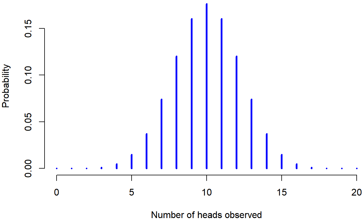
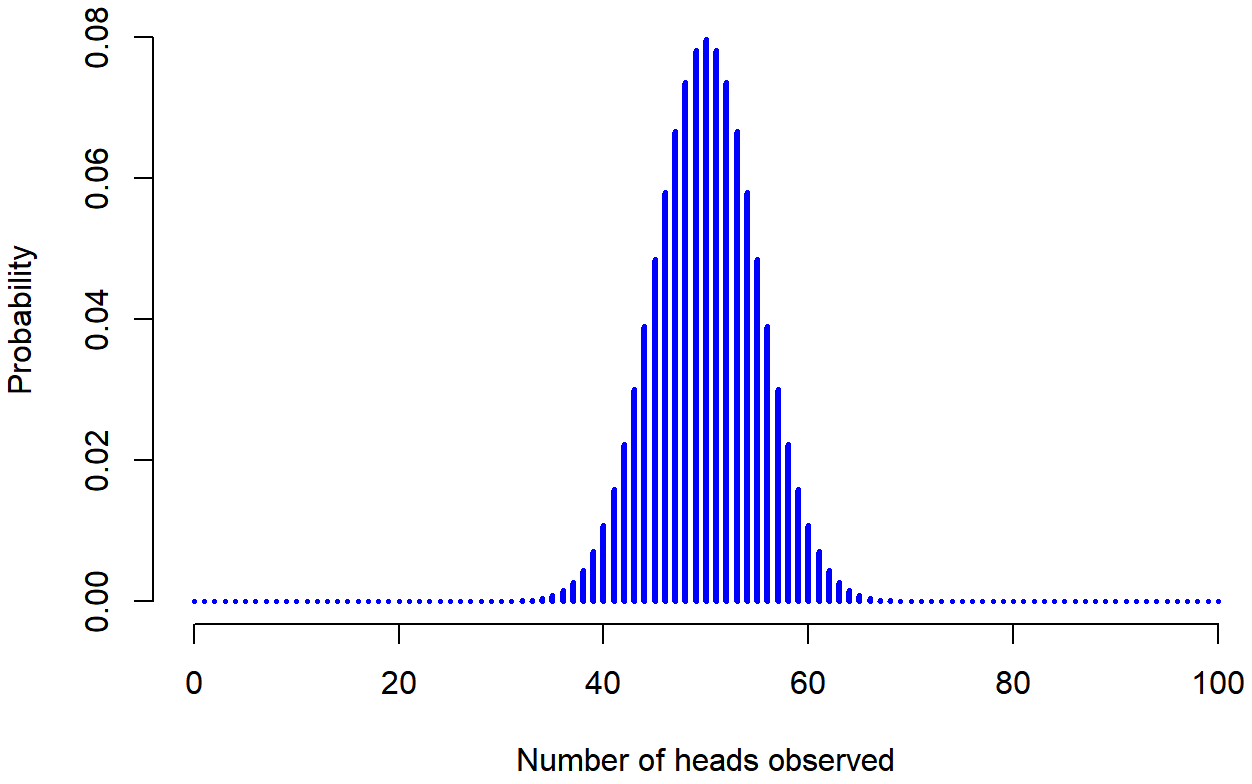
dbinom( x = 4, size = 20, prob = 1/6 )

## [1] 0.2022036

To give you a feel for how the binomial distribution changes when we alter the values of θ and N, let’s suppose that instead of rolling dice, I’m actually flipping coins. This time around, my experiment involves flipping a fair coin repeatedly, and the outcome that I’m interested in is the number of heads that I observe. In this scenario, the success probability is now θ=1/2. Suppose I were to flip the coin N=20 times. In this example, I’ve changed the success probability, but kept the size of the experiment the same. What does this do to our binomial distribution? Well, as Figure 9.4 shows, the main effect of this is to shift the whole distribution, as you’d expect. Okay, what if we flipped a coin N=100 times? Well, in that case, we get Figure 9.5. The distribution stays roughly in the middle, but there’s a bit more variability in the possible outcomes.

Figure 9.4: Two binomial distributions, involving a scenario in which I’m flipping a fair coin, so the underlying success probability is theta=1/2. Here we assume I’m flipping the coin N=20 times.

Figure 9.5: Two binomial distributions, involving a scenario in which I’m flipping a fair coin, so the underlying success probability is theta=1/2. Here we assume that the coin is flipped N=100 times.

knitr::kable(data.frame(stringsAsFactors=FALSE, Binomial = c("$P(X | \\theta, N) = \\displaystyle\\dfrac{N!}{X! (N-X)!}  
\\theta^X (1-\\theta)^{N-X}$"), 
Normal = c("$p(X | \\mu, \\sigma) = \\displaystyle\\dfrac{1}{\\sqrt{2\\pi}\\sigma} \\exp \\left( -\\dfrac{(X - \\mu)^2}
{2\\sigma^2} \\right)$ ")), caption = "Formulas for the binomial and normal distributions. We don't really use these 
formulas for anything in this book, but they're pretty important for more advanced work, so I thought it might be best 
to put them here in a table, where they can't get in the way of the text. In the equation for the binomial, $X!$ is the 
factorial function (i.e., multiply all whole numbers from 1 to $X$), and for the normal distribution \"exp\" refers to 
the exponential function, which we discussed in the Chapter on Data Handling. If these equations don't make a lot of 
sense to you, don't worry too much about them.")

Table 9.2: Formulas for the binomial and normal distributions. We don’t really use these formulas for anything in this book, but they’re pretty important for more advanced work, so I thought it might be best to put them here in a table, where they can’t get in the way of the text. In the equation for the binomial, X! is the factorial function (i.e., multiply all whole numbers from 1 to X), and for the normal distribution “exp” refers to the exponential function, which we discussed in the Chapter on Data Handling. If these equations don’t make a lot of sense to you, don’t worry too much about them.

Binomial	Normal
$$ P(X | \theta, N)=\dfrac{N !}{X !(N-X) !} \theta^{X}(1-\theta)^{N-X} \nonumber$$	$$ p(X | \mu, \sigma)=\dfrac{1}{\sqrt{2 \pi} \sigma} \exp \left(-\dfrac{(X-\mu)^{2}}{2 \sigma^{2}}\right) \nonumber$$

Table 9.3: The naming system for R probability distribution functions. Every probability distribution implemented in R is actually associated with four separate functions, and there is a pretty standardised way for naming these functions.

What.it.does	Prefix	Normal.distribution	Binomial.distribution
probability (density) of	d	dnorm()	dbinom()
cumulative probability of	p	dnorm()	pbinom()
generate random number from	r	rnorm()	rbinom()
q qnorm() qbinom()	q	qnorm()	qbinom(

At this point, I should probably explain the name of the dbinom() function. Obviously, the “binom” part comes from the fact that we’re working with the binomial distribution, but the “d” prefix is probably a bit of a mystery. In this section I’ll give a partial explanation: specifically, I’ll explain why there is a prefix. As for why it’s a “d” specifically, you’ll have to wait until the next section. What’s going on here is that R actually provides four functions in relation to the binomial distribution. These four functions are dbinom(), pbinom(), rbinom() and qbinom(), and each one calculates a different quantity of interest. Not only that, R does the same thing for every probability distribution that it implements. No matter what distribution you’re talking about, there’s a d function, a p function, a q function and a r function. This is illustrated in Table 9.3, using the binomial distribution and the normal distribution as examples.

Let’s have a look at what all four functions do. Firstly, all four versions of the function require you to specify the size and prob arguments: no matter what you’re trying to get R to calculate, it needs to know what the parameters are. However, they differ in terms of what the other argument is, and what the output is. So let’s look at them one at a time.

• The d form we’ve already seen: you specify a particular outcome x, and the output is the probability of obtaining exactly that outcome. (the “d” is short for density, but ignore that for now).
• The p form calculates the cumulative probability. You specify a particular quantile q, and it tells you the probability of obtaining an outcome smaller than or equal to q.
• The q form calculates the quantiles of the distribution. You specify a probability value p, and gives you the corresponding percentile. That is, the value of the variable for which there’s a probability p of obtaining an outcome lower than that value.
• The r form is a random number generator: specifically, it generates n random outcomes from the distribution.

This is a little abstract, so let’s look at some concrete examples. Again, we’ve already covered dbinom() so let’s focus on the other three versions. We’ll start with pbinom(), and we’ll go back to the skull-dice example. Again, I’m rolling 20 dice, and each die has a 1 in 6 chance of coming up skulls. Suppose, however, that I want to know the probability of rolling 4 or fewer skulls. If I wanted to, I could use the dbinom() function to calculate the exact probability of rolling 0 skulls, 1 skull, 2 skulls, 3 skulls and 4 skulls and then add these up, but there’s a faster way. Instead, I can calculate this using the pbinom() function. Here’s the command:

pbinom( q= 4, size = 20, prob = 1/6)

## [1] 0.7687492

In other words, there is a 76.9% chance that I will roll 4 or fewer skulls. Or, to put it another way, R is telling us that a value of 4 is actually the 76.9th percentile of this binomial distribution.

Next, let’s consider the qbinom() function. Let’s say I want to calculate the 75th percentile of the binomial distribution. If we’re sticking with our skulls example, I would use the following command to do this:

qbinom( p = 0.75, size = 20, prob = 1/6)

## [1] 4

Hm. There’s something odd going on here. Let’s think this through. What the qbinom() function appears to be telling us is that the 75th percentile of the binomial distribution is 4, even though we saw from the pbinom() function that 4 is actually the 76.9th percentile. And it’s definitely the pbinom() function that is correct. I promise. The weirdness here comes from the fact that our binomial distribution doesn’t really have a 75th percentile. Not really. Why not? Well, there’s a 56.7% chance of rolling 3 or fewer skulls (you can type pbinom(3, 20, 1/6) to confirm this if you want), and a 76.9% chance of rolling 4 or fewer skulls. So there’s a sense in which the 75th percentile should lie “in between” 3 and 4 skulls. But that makes no sense at all! You can’t roll 20 dice and get 3.9 of them come up skulls. This issue can be handled in different ways: you could report an in between value (or interpolated value, to use the technical name) like 3.9, you could round down (to 3) or you could round up (to 4). The qbinom() function rounds upwards: if you ask for a percentile that doesn’t actually exist (like the 75th in this example), R finds the smallest value for which the the percentile rank is at least what you asked for. In this case, since the “true” 75th percentile (whatever that would mean) lies somewhere between 3 and 4 skulls, R rounds up and gives you an answer of 4. This subtlety is tedious, I admit, but thankfully it’s only an issue for discrete distributions like the binomial (see Section 2.2.5 for a discussion of continuous versus discrete). The other distributions that I’ll talk about (normal, t, χ² and F) are all continuous, and so R can always return an exact quantile whenever you ask for it.

Finally, we have the random number generator. To use the rbinom() function, you specify how many times R should “simulate” the experiment using the n argument, and it will generate random outcomes from the binomial distribution. So, for instance, suppose I were to repeat my die rolling experiment 100 times. I could get R to simulate the results of these experiments by using the following command:

rbinom( n = 100, size = 20, prob = 1/6 )

##   [1] 3 3 3 2 3 3 3 2 3 3 6 2 5 3 1 1 4 7 5 3 3 6 3 4 3 4 5 3 3 3 7 4 5 1 2
##  [36] 1 2 4 2 5 5 4 4 3 1 3 0 2 3 2 2 2 2 1 3 4 5 0 3 2 5 1 2 3 1 5 2 4 3 2
##  [71] 1 2 1 5 2 3 3 2 3 3 4 2 1 2 6 2 3 2 3 3 6 2 1 1 3 3 1 5 4 3

As you can see, these numbers are pretty much what you’d expect given the distribution shown in Figure 9.3. Most of the time I roll somewhere between 1 to 5 skulls. There are a lot of subtleties associated with random number generation using a computer,¹⁴⁴ but for the purposes of this book we don’t need to worry too much about them.