
4.13: Estimating population parameters
- Page ID
- 16789

Let’s pause for a moment to get our bearings. We’re about to go into the topic of estimation. What is that, and why should you care? First, population parameters are things about a distribution. For example, distributions have means. The mean is a parameter of the distribution. The standard deviation of a distribution is a parameter. Anything that can describe a distribution is a potential parameter.
OK fine, who cares? This I think, is a really good question. There are some good concrete reasons to care. And there are some great abstract reasons to care. Unfortunately, most of the time in research, it’s the abstract reasons that matter most, and these can be the most difficult to get your head around.
Concrete population parameters
First some concrete reasons. There are real populations out there, and sometimes you want to know the parameters of them. For example, if you are a shoe company, you would want to know about the population parameters of feet size. As a first pass, you would want to know the mean and standard deviation of the population. If your company knew this, and other companies did not, your company would do better (assuming all shoes are made equal). Why would your company do better, and how could it use the parameters? Here’s one good reason. As a shoe company you want to meet demand with the right amount of supply. If you make too many big or small shoes, and there aren’t enough people to buy them, then you’re making extra shoes that don’t sell. If you don’t make enough of the most popular sizes, you’ll be leaving money on the table. Right? Yes. So, what would be an optimal thing to do? Perhaps, you would make different amounts of shoes in each size, corresponding to how the demand for each shoe size. You would know something about the demand by figuring out the frequency of each size in the population. You would need to know the population parameters to do this.
Fortunately, it’s pretty easy to get the population parameters without measuring the entire population. Who has time to measure every-bodies feet? Nobody, that’s who. Instead, you would just need to randomly pick a bunch of people, measure their feet, and then measure the parameters of the sample. If you take a big enough sample, we have learned that the sample mean gives a very good estimate of the population mean. We will learn shortly that a version of the standard deviation of the sample also gives a good estimate of the standard deviation of the population. Perhaps shoe-sizes have a slightly different shape than a normal distribution. Here too, if you collect a big enough sample, the shape of the distribution of the sample will be a good estimate of the shape of the populations. All of these are good reasons to care about estimating population parameters. But, do you run a shoe company? Probably not.
Abstract population parameters
Even when we think we are talking about something concrete in Psychology, it often gets abstract right away. Instead of measuring the population of feet-sizes, how about the population of human happiness. We all think we know what happiness is, everyone has more or less of it, there are a bunch of people, so there must be a population of happiness right? Perhaps, but it’s not very concrete. The first problem is figuring out how to measure happiness. Let’s use a questionnaire. Consider these questions:
How happy are you right now on a scale from 1 to 7? How happy are you in general on a scale from 1 to 7? How happy are you in the mornings on a scale from 1 to 7? How happy are you in the afternoons on a scale from 1 to 7?
- = very unhappy
- = unhappy
- = sort of unhappy
- = in the middle
- = sort of happy
- = happy
- = very happy
Forget about asking these questions to everybody in the world. Let’s just ask them to lots of people (our sample). What do you think would happen? Well, obviously people would give all sorts of answers right. We could tally up the answers and plot them in a histogram. This would show us a distribution of happiness scores from our sample. “Great, fantastic!”, you say. Yes, fine and dandy.
So, on the one hand we could say lots of things about the people in our sample. We could say exactly who says they are happy and who says they aren’t, after all they just told us!
But, what can we say about the larger population? Can we use the parameters of our sample (e.g., mean, standard deviation, shape etc.) to estimate something about a larger population. Can we infer how happy everybody else is, just from our sample? HOLD THE PHONE.
Complications with inference
Before listing a bunch of complications, let me tell you what I think we can do with our sample. Provided it is big enough, our sample parameters will be a pretty good estimate of what another sample would look like. Because of the following discussion, this is often all we can say. But, that’s OK, as you see throughout this book, we can work with that!
Problem 1: Multiple populations: If you looked at a large sample of questionnaire data you will find evidence of multiple distributions inside your sample. People answer questions differently. Some people are very cautious and not very extreme. Their answers will tend to be distributed about the middle of the scale, mostly 3s, 4s, and 5s. Some people are very bi-modal, they are very happy and very unhappy, depending on time of day. These people’s answers will be mostly 1s and 2s, and 6s and 7s, and those numbers look like they come from a completely different distribution. Some people are entirely happy or entirely unhappy. Again, these two “populations” of people’s numbers look like two different distributions, one with mostly 6s and 7s, and one with mostly 1s and 2s. Other people will be more random, and their scores will look like a uniform distribution. So, is there a single population with parameters that we can estimate from our sample? Probably not. Could be a mixture of lots of populations with different distributions.
Problem 2: What do these questions measure?: If the whole point of doing the questionnaire is to estimate the population’s happiness, we really need wonder if the sample measurements actually tell us anything about happiness in the first place. Some questions: Are people accurate in saying how happy they are? Does the measure of happiness depend on the scale, for example, would the results be different if we used 0-100, or -100 to +100, or no numbers? Does the measure of happiness depend on the wording in the question? Does a measure like this one tell us everything we want to know about happiness (probably not), what is it missing (who knows? probably lots). In short, nobody knows if these kinds of questions measure what we want them to measure. We just hope that they do. Instead, we have a very good idea of the kinds of things that they actually measure. It’s really quite obvious, and staring you in the face. Questionnaire measurements measure how people answer questionnaires. In other words, how people behave and answer questions when they are given a questionnaire. This might also measure something about happiness, when the question has to do about happiness. But, it turns out people are remarkably consistent in how they answer questions, even when the questions are total nonsense, or have no questions at all (just numbers to choose!) Maul (2017).
The take home complications here are that we can collect samples, but in Psychology, we often don’t have a good idea of the populations that might be linked to these samples. There might be lots of populations, or the populations could be different depending on who you ask. Finally, the “population” might not be the one you want it to be.
Experiments and Population parameters
OK, so we don’t own a shoe company, and we can’t really identify the population of interest in Psychology, can’t we just skip this section on estimation? After all, the “population” is just too weird and abstract and useless and contentious. HOLD THE PHONE AGAIN!
It turns out we can apply the things we have been learning to solve lots of important problems in research. These allow us to answer questions with the data that we collect. Parameter estimation is one of these tools. We just need to be a little bit more creative, and a little bit more abstract to use the tools.
Here is what we know already. The numbers that we measure come from somewhere, we have called this place “distributions”. Distributions control how the numbers arrive. Some numbers happen more than others depending on the distribution. We assume, even if we don’t know what the distribution is, or what it means, that the numbers came from one. Second, when get some numbers, we call it a sample. This entire chapter so far has taught you one thing. When your sample is big, it resembles the distribution it came from. And, when your sample is big, it will resemble very closely what another big sample of the same thing will look like. We can use this knowledge!
Very often as Psychologists what we want to know is what causes what. We want to know if X causes something to change in Y. Does eating chocolate make you happier? Does studying improve your grades? There a bazillions of these kinds of questions. And, we want answers to them.
I’ve been trying to be mostly concrete so far in this textbook, that’s why we talk about silly things like chocolate and happiness, at least they are concrete. Let’s give a go at being abstract. We can do it.
So, we want to know if X causes Y to change. What is X? What is Y? X is something you change, something you manipulate, the independent variable. Y is something you measure. So, we will be taking samples from Y. “Oh I get it, we’ll take samples from Y, then we can use the sample parameters to estimate the population parameters of Y!” NO, not really, but yes sort of. We will take sample from Y, that is something we absolutely do. In fact, that is really all we ever do, which is why talking about the population of Y is kind of meaningless. We’re more interested in our samples of Y, and how they behave.
So, what would happen if we removed X from the universe altogether, and then took a big sample of Y. We’ll pretend Y measures something in a Psychology experiment. So, we know right away that Y is variable. When we take a big sample, it will have a distribution (because Y is variable). So, we can do things like measure the mean of Y, and measure the standard deviation of Y, and anything else we want to know about Y. Fine. What would happen if we replicated this measurement. That is, we just take another random sample of Y, just as big as the first. What should happen is that our first sample should look a lot like our second example. After all, we didn’t do anything to Y, we just took two big samples twice. Both of our samples will be a little bit different (due to sampling error), but they’ll be mostly the same. The bigger our samples, the more they will look the same, especially when we don’t do anything to cause them to be different. In other words, we can use the parameters of one sample to estimate the parameters of a second sample, because they will tend to be the same, especially when they are large.
We are now ready for step two. You want to know if X changes Y. What do you do? You make X go up and take a big sample of Y then look at it. You make X go down, then take a second big sample of Y and look at it. Next, you compare the two samples of Y. If X does nothing then what should you find? We already discussed that in the previous paragraph. If X does nothing, then both of your big samples of Y should be pretty similar. However, if X does something to Y, then one of your big samples of Y will be different from the other. You will have changed something about Y. Maybe X makes the mean of Y change. Or maybe X makes the variation in Y change. Or, maybe X makes the whole shape of the distribution change. If we find any big changes that can’t be explained by sampling error, then we can conclude that something about X caused a change in Y! We could use this approach to learn about what causes what!
The very important idea is still about estimation, just not population parameter estimation exactly. We know that when we take samples they naturally vary. So, when we estimate a parameter of a sample, like the mean, we know we are off by some amount. When we find that two samples are different, we need to find out if the size of the difference is consistent with what sampling error can produce, or if the difference is bigger than that. If the difference is bigger, then we can be confident that sampling error didn’t produce the difference. So, we can confidently infer that something else (like an X) did cause the difference. This bit of abstract thinking is what most of the rest of the textbook is about. Determining whether there is a difference caused by your manipulation. There’s more to the story, there always is. We can get more specific than just, is there a difference, but for introductory purposes, we will focus on the finding of differences as a foundational concept.
Interim summary
We’ve talked about estimation without doing any estimation, so in the next section we will do some estimating of the mean and of the standard deviation. Formally, we talk about this as using a sample to estimate a parameter of the population. Feel free to think of the “population” in different ways. It could be concrete population, like the distribution of feet-sizes. Or, it could be something more abstract, like the parameter estimate of what samples usually look like when they come from a distribution.
Estimating the population mean
Suppose we go to Brooklyn and 100 of the locals are kind enough to sit through an IQ test. The average IQ score among these people turns out to be \(\bar{X}=98.5\). So what is the true mean IQ for the entire population of Brooklyn? Obviously, we don’t know the answer to that question. It could be \(97.2\), but if could also be \(103.5\). Our sampling isn’t exhaustive so we cannot give a definitive answer. Nevertheless if forced to give a “best guess” I’d have to say \(98.5\). That’s the essence of statistical estimation: giving a best guess. We’re using the sample mean as the best guess of the population mean.
In this example, estimating the unknown population parameter is straightforward. I calculate the sample mean, and I use that as my estimate of the population mean. It’s pretty simple, and in the next section we’ll explain the statistical justification for this intuitive answer. However, for the moment let’s make sure you recognize that the sample statistic and the estimate of the population parameter are conceptually different things. A sample statistic is a description of your data, whereas the estimate is a guess about the population. With that in mind, statisticians often use different notation to refer to them. For instance, if true population mean is denoted \(\mu\), then we would use \(\hat\mu\) to refer to our estimate of the population mean. In contrast, the sample mean is denoted \(\bar{X}\) or sometimes \(m\). However, in simple random samples, the estimate of the population mean is identical to the sample mean: if I observe a sample mean of \(\bar{X} = 98.5\), then my estimate of the population mean is also \(\hat\mu = 98.5\). To help keep the notation clear, here’s a handy table:
| Symbol | What is it? | Do we know what it is? |
|---|---|---|
| \(\bar{X}\) | Sample mean | Yes, calculated from the raw data |
| \(\mu\) | True population mean | Almost never known for sure |
| \(\hat{\mu}\) | Estimate of the population mean | Yes, identical to the sample mean |
Estimating the population standard deviation
So far, estimation seems pretty simple, and you might be wondering why I forced you to read through all that stuff about sampling theory. In the case of the mean, our estimate of the population parameter (i.e. \(\hat\mu\)) turned out to identical to the corresponding sample statistic (i.e. \(\bar{X}\)). However, that’s not always true. To see this, let’s have a think about how to construct an estimate of the population standard deviation, which we’ll denote \(\hat\sigma\). What shall we use as our estimate in this case? Your first thought might be that we could do the same thing we did when estimating the mean, and just use the sample statistic as our estimate. That’s almost the right thing to do, but not quite.
Here’s why. Suppose I have a sample that contains a single observation. For this example, it helps to consider a sample where you have no intuitions at all about what the true population values might be, so let’s use something completely fictitious. Suppose the observation in question measures the cromulence of my shoes. It turns out that my shoes have a cromulence of 20. So here’s my sample:
20
This is a perfectly legitimate sample, even if it does have a sample size of \(N=1\). It has a sample mean of 20, and because every observation in this sample is equal to the sample mean (obviously!) it has a sample standard deviation of 0. As a description of the sample this seems quite right: the sample contains a single observation and therefore there is no variation observed within the sample. A sample standard deviation of \(s = 0\) is the right answer here. But as an estimate of the population standard deviation, it feels completely insane, right? Admittedly, you and I don’t know anything at all about what “cromulence” is, but we know something about data: the only reason that we don’t see any variability in the sample is that the sample is too small to display any variation! So, if you have a sample size of \(N=1\), it feels like the right answer is just to say “no idea at all”.
Notice that you don’t have the same intuition when it comes to the sample mean and the population mean. If forced to make a best guess about the population mean, it doesn’t feel completely insane to guess that the population mean is 20. Sure, you probably wouldn’t feel very confident in that guess, because you have only the one observation to work with, but it’s still the best guess you can make.
Let’s extend this example a little. Suppose I now make a second observation. My data set now has \(N=2\) observations of the cromulence of shoes, and the complete sample now looks like this:
20, 22
This time around, our sample is just large enough for us to be able to observe some variability: two observations is the bare minimum number needed for any variability to be observed! For our new data set, the sample mean is \(\bar{X}=21\), and the sample standard deviation is \(s=1\). What intuitions do we have about the population? Again, as far as the population mean goes, the best guess we can possibly make is the sample mean: if forced to guess, we’d probably guess that the population mean cromulence is 21. What about the standard deviation? This is a little more complicated. The sample standard deviation is only based on two observations, and if you’re at all like me you probably have the intuition that, with only two observations, we haven’t given the population “enough of a chance” to reveal its true variability to us. It’s not just that we suspect that the estimate is wrong: after all, with only two observations we expect it to be wrong to some degree. The worry is that the error is systematic.
If the error is systematic, that means it is biased. For example, imagine if the sample mean was always smaller than the population mean. If this was true (it’s not), then we couldn’t use the sample mean as an estimator. It would be biased, we’d be using the wrong number.
It turns out the sample standard deviation is a biased estimator of the population standard deviation. We can sort of anticipate this by what we’ve been discussing. When the sample size is 1, the standard deviation is 0, which is obviously to small. When the sample size is 2, the standard deviation becomes a number bigger than 0, but because we only have two sample, we suspect it might still be too small. Turns out this intuition is correct.
It would be nice to demonstrate this somehow. There are in fact mathematical proofs that confirm this intuition, but unless you have the right mathematical background they don’t help very much. Instead, what I’ll do is use R to simulate the results of some experiments. With that in mind, let’s return to our IQ studies. Suppose the true population mean IQ is 100 and the standard deviation is 15. I can use the rnorm() function to generate the the results of an experiment in which I measure \(N=2\) IQ scores, and calculate the sample standard deviation. If I do this over and over again, and plot a histogram of these sample standard deviations, what I have is the sampling distribution of the standard deviation. I’ve plotted this distribution in Figure \(\PageIndex{1}\).
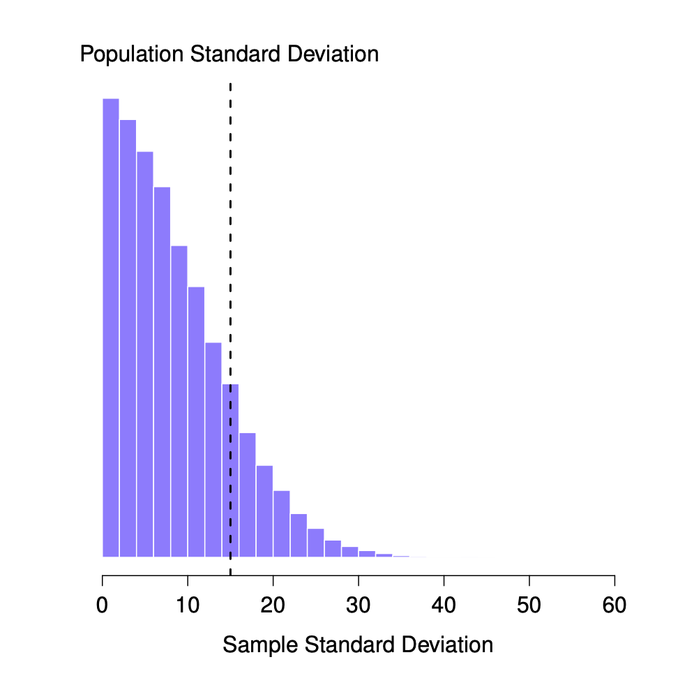
Even though the true population standard deviation is 15, the average of the sample standard deviations is only 8.5. Notice that this is a very different from when we were plotting sampling distributions of the sample mean, those were always centered around the mean of the population.
Now let’s extend the simulation. Instead of restricting ourselves to the situation where we have a sample size of \(N=2\), let’s repeat the exercise for sample sizes from 1 to 10. If we plot the average sample mean and average sample standard deviation as a function of sample size, you get the following results.
Figure \(\PageIndex{2}\) shows the sample mean as a function of sample size. Notice it’s a flat line. The sample mean doesn’t underestimate or overestimate the population mean. It is an unbiased estimate!
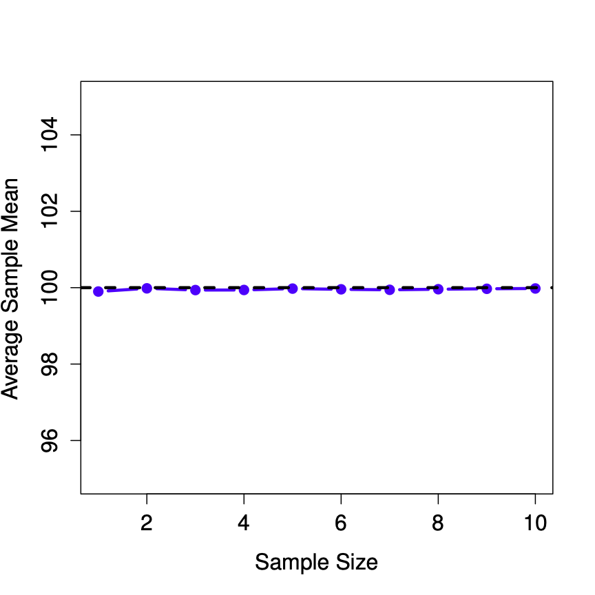
Figure \(\PageIndex{3}\) shows the sample standard deviation as a function of sample size. Notice it is not a flat line. The sample standard deviation systematically underestimates the population standard deviation!
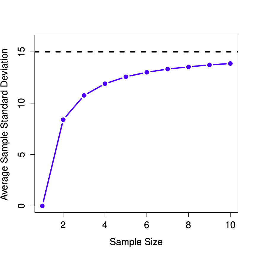
In other words, if we want to make a “best guess” (\(\hat\sigma\), our estimate of the population standard deviation) about the value of the population standard deviation \(\sigma\), we should make sure our guess is a little bit larger than the sample standard deviation \(s\).
The fix to this systematic bias turns out to be very simple. Here’s how it works. Before tackling the standard deviation, let’s look at the variance. If you recall from the second chapter, the sample variance is defined to be the average of the squared deviations from the sample mean. That is:
\[s^2 = \frac{1}{N} \sum_{i=1}^N (X_i - \bar{X})^2 \nonumber \]
The sample variance \(s^2\) is a biased estimator of the population variance \(\sigma^2\). But as it turns out, we only need to make a tiny tweak to transform this into an unbiased estimator. All we have to do is divide by \(N-1\) rather than by \(N\). If we do that, we obtain the following formula:
\[\hat\sigma^2 = \frac{1}{N-1} \sum_{i=1}^N (X_i - \bar{X})^2 \nonumber \]
This is an unbiased estimator of the population variance \(\sigma\).
A similar story applies for the standard deviation. If we divide by \(N-1\) rather than \(N\), our estimate of the population standard deviation becomes:
\[\hat\sigma = \sqrt{\frac{1}{N-1} \sum_{i=1}^N (X_i - \bar{X})^2} \nonumber \]
It is worth pointing out that software programs make assumptions for you, about which variance and standard deviation you are computing. Some programs automatically divide by \(N-1\), some do not. You need to check to figure out what they are doing. Don’t let the software tell you what to do. Software is for you telling it what to do.
One final point: in practice, a lot of people tend to refer to \(\hat{\sigma}\) (i.e., the formula where we divide by \(N-1\)) as the sample standard deviation. Technically, this is incorrect: the sample standard deviation should be equal to \(s\) (i.e., the formula where we divide by \(N\)). These aren’t the same thing, either conceptually or numerically. One is a property of the sample, the other is an estimated characteristic of the population. However, in almost every real life application, what we actually care about is the estimate of the population parameter, and so people always report \(\hat\sigma\) rather than \(s\).
Note, whether you should divide by N or N-1 also depends on your philosophy about what you are doing. For example, if you don’t think that what you are doing is estimating a population parameter, then why would you divide by N-1? Also, when N is large, it doesn’t matter too much. The difference between a big N, and a big N-1, is just -1.
This is the right number to report, of course, it’s that people tend to get a little bit imprecise about terminology when they write it up, because “sample standard deviation” is shorter than “estimated population standard deviation”. It’s no big deal, and in practice I do the same thing everyone else does. Nevertheless, I think it’s important to keep the two concepts separate: it’s never a good idea to confuse “known properties of your sample” with “guesses about the population from which it came”. The moment you start thinking that \(s\) and \(\hat\sigma\) are the same thing, you start doing exactly that.
To finish this section off, here’s another couple of tables to help keep things clear:
| Symbol | What is it? | Do we know what it is? |
|---|---|---|
| \(s^2\) | Sample variance | Yes, calculated from the raw data |
| \(\sigma^2\) | Population variance | Almost never known for sure |
| \(\hat{\sigma}^2\) | Estimate of the population variance | Yes, but not the same as the sample variance |