6.3: Using Standard Error for Probability

We saw in chapter 6 that we can use \(z\)-scores to split up a normal distribution and calculate the proportion of the area under the curve in one of the new regions, giving us the probability of randomly selecting a \(z\)-score in that range. We can follow the exact sample process for sample means, converting them into \(z\)-scores and calculating probabilities. The only difference is that instead of dividing a raw score by the standard deviation, we divide the sample mean by the standard error.

\[z=\dfrac{\overline{X}-\mu}{\sigma_{\overline{X}}}=\dfrac{\overline{X}-\mu}{\frac {\overline{\sigma}}{\sqrt{n}}} \]

Let’s say we are drawing samples from a population with a mean of 50 and standard deviation of 10 (the same values used in Figure 2). What is the probability that we get a random sample of size 10 with a mean greater than or equal to 55? That is, for n = 10, what is the probability that \(\overline{X}\) ≥ 55? First, we need to convert this sample mean score into a \(z\)-score:

\[z=\dfrac{55-50}{\frac{10}{\sqrt{10}}}=\dfrac{5}{3.16}=1.58 \nonumber \]

Now we need to shade the area under the normal curve corresponding to scores greater than \(z\) = 1.58 as in Figure \(\PageIndex{1}\):

Figure \(\PageIndex{1}\): Area under the curve greater than \(z\) = 1.58

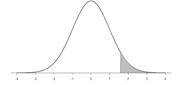
Now we go to our \(z\)-table and find that the area to the left of \(z\) = 1.58 is 0.9429. Finally, because we need the area to the right (per our shaded diagram), we simply subtract this from 1 to get 1.00 – 0.9429 = 0.0571. So, the probability of randomly drawing a sample of 10 people from a population with a mean of 50 and standard deviation of 10 whose sample mean is 55 or more is \(p\) = .0571, or 5.71%. Notice that we are talking about means that are 55 or more. That is because, strictly speaking, it’s impossible to calculate the probability of a score taking on exactly 1 value since the “shaded region” would just be a line with no area to calculate.

Now let’s do the same thing, but assume that instead of only having a sample of 10 people we took a sample of 50 people. First, we find \(z\):

\[z=\dfrac{55-50}{\frac{10}{\sqrt{50}}}=\dfrac{5}{1.41}=3.55 \]

Then we shade the appropriate region of the normal distribution:

Figure \(\PageIndex{2}\): Area under the curve greater than \(z\) = 3.55

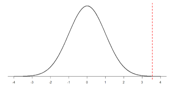
Notice that no region of Figure \(\PageIndex{2}\) appears to be shaded. That is because the area under the curve that far out into the tail is so small that it can’t even be seen (the red line has been added to show exactly where the region starts). Thus, we already know that the probability must be smaller for \(N\) = 50 than \(N\) = 10 because the size of the area (the proportion) is much smaller.

We run into a similar issue when we try to find \(z\) = 3.55 on our Standard Normal Distribution Table. The table only goes up to 3.09 because everything beyond that is almost 0 and changes so little that it’s not worth printing values. The closest we can get is subtracting the largest value, 0.9990, from 1 to get 0.001. We know that, technically, the actual probability is smaller than this (since 3.55 is farther into the tail than 3.09), so we say that the probability is \(p\) < 0.001, or less than 0.1%.

This example shows what an impact sample size can have. From the same population, looking for exactly the same thing, changing only the sample size took us from roughly a 5% chance (or about 1/20 odds) to a less than 0.1% chance (or less than 1 in 1000). As the sample size n increased, the standard error decreased, which in turn caused the value of \(z\) to increase, which finally caused the \(p\)-value (a term for probability we will use a lot in Unit 2) to decrease. You can think of this relation like gears: turning the first gear (sample size) clockwise causes the next gear (standard error) to turn counterclockwise, which causes the third gear (z) to turn clockwise, which finally causes the last gear (probability) to turn counterclockwise. All of these pieces fit together, and the relations will always be the same:

\[\mathrm{n} \uparrow \sigma_{\overline{X}} \downarrow \mathrm{z} \uparrow \mathrm{p} \downarrow\]

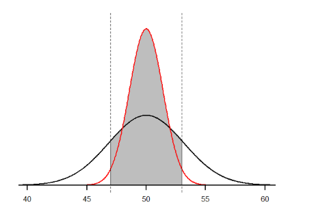
Let’s look at this one more way. For the same population of sample size 50 and standard deviation 10, what proportion of sample means fall between 47 and 53 if they are of sample size 10 and sample size 50?

We’ll start again with \(n\) = 10. Converting 47 and 53 into \(z\)-scores, we get \(z\) = -0.95 and \(z\) = 0.95, respectively. From our \(z\)-table, we find that the proportion between these two scores is 0.6578 (the process here is left off for the student to practice converting \(\overline{X}\) to \(z\) and \(z\) to proportions). So, 65.78% of sample means of sample size 10 will fall between 47 and 53. For \(n\) = 50, our \(z\)-scores for 47 and 53 are ±2.13, which gives us a proportion of the area as 0.9668, almost 97%! Shaded regions for each of these sampling distributions is displayed in Figure \(\PageIndex{3}\). The sampling distributions are shown on the original scale, rather than as z-scores, so you can see the effect of the shading and how much of the body falls into the range, which is marked off with dotted line.

Figure \(\PageIndex{3}\): Areas between 47 and 53 for sampling distributions of \(n\) = 10 and \(n\) = 50