
4.2: Z-scores
- Page ID
- 7098

A \(z\)-score is a standardized version of a raw score (\(x\)) that gives information about the relative location of that score within its distribution. The formula for converting a raw score into a \(z\)-score is:
\[z=\dfrac{x-\mu}{\sigma} \]
for values from a population and for values from a sample:
\[z=\dfrac{x-\overline{X}}{s} \]
As you can see, \(z\)-scores combine information about where the distribution is located (the mean/center) with how wide the distribution is (the standard deviation/spread) to interpret a raw score (\(x\)). Specifically, \(z\)-scores will tell us how far the score is away from the mean in units of standard deviations and in what direction.
The value of a \(z\)-score has two parts: the sign (positive or negative) and the magnitude (the actual number). The sign of the \(z\)-score tells you in which half of the distribution the z-score falls: a positive sign (or no sign) indicates that the score is above the mean and on the right hand-side or upper end of the distribution, and a negative sign tells you the score is below the mean and on the left-hand side or lower end of the distribution. The magnitude of the number tells you, in units of standard deviations, how far away the score is from the center or mean. The magnitude can take on any value between negative and positive infinity, but for reasons we will see soon, they generally fall between -3 and 3.
Let’s look at some examples. A \(z\)-score value of -1.0 tells us that this z-score is 1 standard deviation (because of the magnitude 1.0) below (because of the negative sign) the mean. Similarly, a \(z\)-score value of 1.0 tells us that this \(z\)-score is 1 standard deviation above the mean. Thus, these two scores are the same distance away from the mean but in opposite directions. A \(z\)-score of -2.5 is two-and-a-half standard deviations below the mean and is therefore farther from the center than both of the previous scores, and a \(z\)-score of 0.25 is closer than all of the ones before. In Unit 2, we will learn to formalize the distinction between what we consider “close” to the center or “far” from the center. For now, we will use a rough cut-off of 1.5 standard deviations in either direction as the difference between close scores (those within 1.5 standard deviations or between \(z\) = -1.5 and \(z\) = 1.5) and extreme scores (those farther than 1.5 standard deviations – below \(z\) = -1.5 or above \(z\) = 1.5).
We can also convert raw scores into \(z\)-scores to get a better idea of where in the distribution those scores fall. Let’s say we get a score of 68 on an exam. We may be disappointed to have scored so low, but perhaps it was just a very hard exam. Having information about the distribution of all scores in the class would be helpful to put some perspective on ours. We find out that the class got an average score of 54 with a standard deviation of 8. To find out our relative location within this distribution, we simply convert our test score into a \(z\)-score.
\[z=\dfrac{X-\mu}{\sigma}=\frac{68-54}{8}=1.75 \nonumber \]
We find that we are 1.75 standard deviations above the average, above our rough cut off for close and far. Suddenly our 68 is looking pretty good!
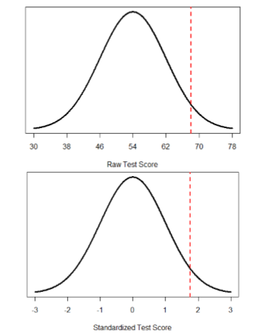
Figure \(\PageIndex{1}\) shows both the raw score and the \(z\)-score on their respective distributions. Notice that the red line indicating where each score lies is in the same relative spot for both. This is because transforming a raw score into a \(z\)-score does not change its relative location, it only makes it easier to know precisely where it is.
\(Z\)-scores are also useful for comparing scores from different distributions. Let’s say we take the SAT and score 501 on both the math and critical reading sections. Does that mean we did equally well on both? Scores on the math portion are distributed normally with a mean of 511 and standard deviation of 120, so our \(z\)-score on the math section is
\[z_{math}=\dfrac{501-511}{120}=-0.08 \nonumber \]
which is just slightly below average (note that use of “math” as a subscript; subscripts are used when presenting multiple versions of the same statistic in order to know which one is which and have no bearing on the actual calculation). The critical reading section has a mean of 495 and standard deviation of 116, so
\[z_{C R}=\frac{501-495}{116}=0.05 \nonumber \]
So even though we were almost exactly average on both tests, we did a little bit better on the critical reading portion relative to other people.
Finally, \(z\)-scores are incredibly useful if we need to combine information from different measures that are on different scales. Let’s say we give a set of employees a series of tests on things like job knowledge, personality, and leadership. We may want to combine these into a single score we can use to rate employees for development or promotion, but look what happens when we take the average of raw scores from different scales, as shown in Table \(\PageIndex{1}\):
| Raw Scores | Job Knowledge (0 – 100) | Personality (1 –5) | Leadership (1 – 5) | Average |
|---|---|---|---|---|
| Employee 1 | 98 | 4.2 | 1.1 | 34.43 |
| Employee 2 | 96 | 3.1 | 4.5 | 34.53 |
| Employee 3 | 97 | 2.9 | 3.6 | 34.50 |
Because the job knowledge scores were so big and the scores were so similar, they overpowered the other scores and removed almost all variability in the average. However, if we standardize these scores into \(z\)-scores, our averages retain more variability and it is easier to assess differences between employees, as shown in Table \(\PageIndex{2}\).
| \(z\)-Scores | Job Knowledge (0 – 100) | Personality (1 –5) | Leadership (1 – 5) | Average |
|---|---|---|---|---|
| Employee 1 | 1.00 | 1.14 | -1.12 | 0.34 |
| Employee 2 | -1.00 | -0.43 | 0.81 | -0.20 |
| Employee 3 | 0.00 | -0.71 | 0.30 | -0.14 |
Setting the scale of a distribution
Another convenient characteristic of \(z\)-scores is that they can be converted into any “scale” that we would like. Here, the term scale means how far apart the scores are (their spread) and where they are located (their central tendency). This can be very useful if we don’t want to work with negative numbers or if we have a specific range we would like to present. The formulas for transforming \(z\) to \(x\) are:
\[x=z \sigma+\mu \]
for a population and
\[x=z s+\overline{X} \]
for a sample. Notice that these are just simple rearrangements of the original formulas for calculating \(z\) from raw scores.
Let’s say we create a new measure of intelligence, and initial calibration finds that our scores have a mean of 40 and standard deviation of 7. Three people who have scores of 52, 43, and 34 want to know how well they did on the measure. We can convert their raw scores into \(z\)-scores:
\[\begin{aligned} z &=\dfrac{52-40}{7}=1.71 \\ z &=\dfrac{43-40}{7}=0.43 \\ z &=\dfrac{34-40}{7}=-0.80 \end{aligned} \nonumber \]
A problem is that these new \(z\)-scores aren’t exactly intuitive for many people. We can give people information about their relative location in the distribution (for instance, the first person scored well above average), or we can translate these \(z\) scores into the more familiar metric of IQ scores, which have a mean of 100 and standard deviation of 16:
\[\begin{array}{l}{\mathrm{IQ}=1.71 * 16+100=127.36} \\ {\mathrm{IQ}=0.43 * 16+100=106.88} \\ {\mathrm{IQ}=-0.80 * 16+100=87.20}\end{array} \nonumber \]
We would also likely round these values to 127, 107, and 87, respectively, for convenience.