1.4: Eliminating Trend and Seasonal Components
- Page ID
- 903
Recall the classical decomposition (1.1.1),
\[
X_t=m_t+s_t+Y_t, \qquad t\in T,
\nonumber \]
with \(E[Y_t]=0\). In this section, three methods are discussed that aim at estimating both the trend and seasonal components in the data. As additional requirement on \((s_t\colon t\in T)\), it is assumed that
\[
s_{t+d}=s_t,\qquad \sum_{j=1}^ds_j=0,
\nonumber \]
where \(d\) denotes the period of the seasonal component. (If dealing with yearly data sampled monthly, then obviously \(d=12\).) It is convenient to relabel the observations \(x_1,\ldots,x_n\) in terms of the seasonal period \(d\) as
\[x_{j,k}=x_{k+d(j-1)}.
\nonumber \]
In the case of yearly data, observation \(x_{j,k}\) thus represents the data point observed for the \(k\)th month of the \(j\)th year. For convenience the data is always referred to in this fashion even if the actual period is something other than 12.
Method 1 (Small trend method) If the changes in the drift term appear to be small, then it is reasonable to assume that the drift in year \(j\), say, \(m_j\) is constant. As a natural estimator one can therefore apply
\[
\hat{m}_j=\frac{1}{d}\sum_{k=1}^dx_{j,k}.
\nonumber \]
To estimate the seasonality in the data, one can in a second step utilize the quantities
\[
\hat{s}_k=\frac 1N\sum_{j=1}^N(x_{j,k}-\hat{m}_j),
\nonumber \]
where \(N\) is determined by the equation \(n=Nd\), provided that data has been collected over \(N\) full cycles. Direct calculations show that these estimators possess the property \(\hat{s}_1+\ldots+\hat{s}_d=0\) (as in the case of the true seasonal components \(s_t\)). To further assess the quality of the fit, one needs to analyze the observed residuals
\[
\hat{y}_{j,k}=x_{j,k}-\hat{m}_j-\hat{s}_k.
\nonumber \]
Note that due to the relabeling of the observations and the assumption of a slowly changing trend, the drift component is solely described by the "annual'' subscript \(j\), while the seasonal component only contains the "monthly'' subscript \(k\).
-
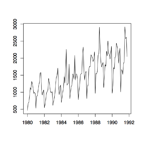
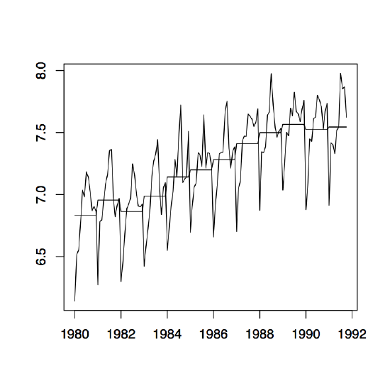
Figure 1.10: Time series plots of the red wine sales in Australia from January 1980 to October 1991 (left) and its log transformation with yearly mean estimates (right).
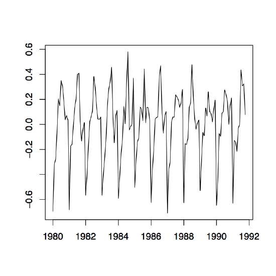
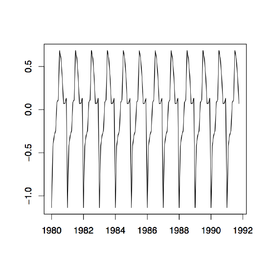
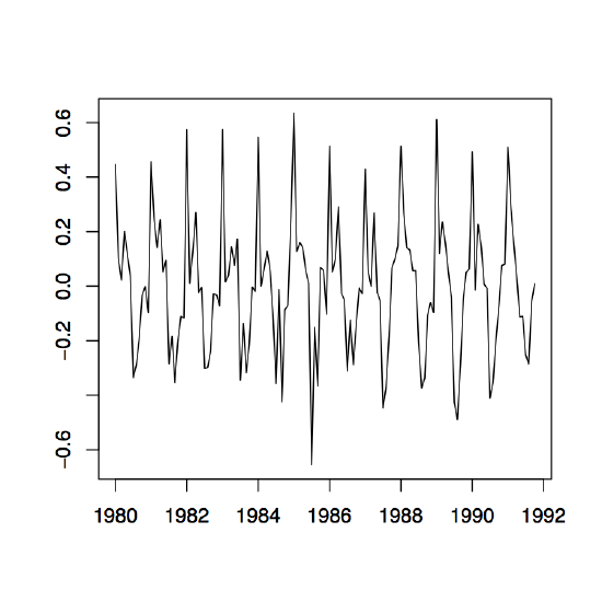
Example 1.4.1 (Australian Wine Sales). The left panel of Figure 1.10 shows the monthly sales of red wine (in kiloliters) in Australia from January 1980 to October 1991. Since there is an apparent increase in the fluctuations over time, the right panel of the same figure shows the natural logarithm transform of the data. There is clear evidence of both trend and seasonality. In the following, the log transformed data is studied. Using the small trend method as described above, the annual means are estimated first. They are already incorporated in the right time series plot of Figure 1.10. Note that there are only ten months of data available for the year 1991, so that the estimation has to be adjusted accordingly. The detrended data is shown in the left panel of Figure 1.11. The middle plot in the same figure shows the estimated seasonal component, while the right panel displays the residuals. Even though the assumption of small changes in the drift is somewhat questionable, the residuals appear to look quite nice. They indicate that there is dependence in the data (see Section 1.5 below for more on this subject).
-
Figure 1.11: The detrended log series (left), the estimated seasonal component (center) and the corresponding residuals series (right) of the Australian red wine sales data.
Method 2 (Moving average estimation) This method is to be preferred over the first one whenever the underlying trend component cannot be assumed constant. Three steps are to be applied to the data.
1st Step: Trend estimation. At first, focus on the removal of the trend component with the linear filters discussed in the previous section. If the period \(d\) is odd, then one can directly use \(\hat{m}_t=W_t\) as in (1.3.2) with \(q\) specified by the equation \(d=2q+1\). If the period \(d=2q\) is even, then slightly modify \(W_t\) and use
\[
\hat{m}_t=\frac 1d(.5x_{t-q}+x_{t-q+1}+\ldots+x_{t+q-1}+.5x_{t+q}),
\qquad t=q+1,\ldots,n-q.
\nonumber \]
2nd Step: Seasonality estimation. To estimate the seasonal component, let
\begin{align*}
\mu_k&=\frac 1{N-1}\sum_{j=2}^N(x_{k+d(j-1)}-\hat{m}_{k+d(j-1)}),
\qquad k=1,\ldots,q,\\[.2cm]
\mu_k&=\frac 1{N-1}\sum_{j=1}^{N-1}(x_{k+d(j-1)}-\hat{m}_{k+d(j-1)}),
\qquad k=q+1,\ldots,d.
\end{align*}
Define now
\[
\hat{s}_k=\mu_k-\frac 1d\sum_{\ell=1}^d\mu_\ell,\qquad k=1,\ldots,d,
\nonumber \]
and set \(\hat{s}_{k}=\hat{s}_{k-d}\) whenever \(k>d\). This will provide us with deseasonalized data which can be examined further. In the final step, any remaining trend can be removed from the data.
3rd Step: Trend Reestimation. Apply any of the methods from Section 1.3.
Method 3 (Differencing at lag d) Introducing the lag-d difference operator \(\nabla_d\), defined by letting
\[
\nabla_dX_t=X_t-X_{t-d}=(1-B^d)X_t,\qquad t=d+1,\ldots,n,
\nonumber \]
and assuming model (1.1.1), one arrives at the transformed random variables
\[
\nabla_dX_t=m_t-m_{t-d}+Y_t-Y_{t-d},\qquad t=d+1,\ldots,n.
\nonumber \]
Note that the seasonality is removed, since \(s_t=s_{t-d}\). The remaining noise variables \(Y_t-Y_{t-d}\) are stationary and have zero mean. The new trend component \(m_t-m_{t-d}\) can be eliminated using any of the methods developed in Section 1.3.
-
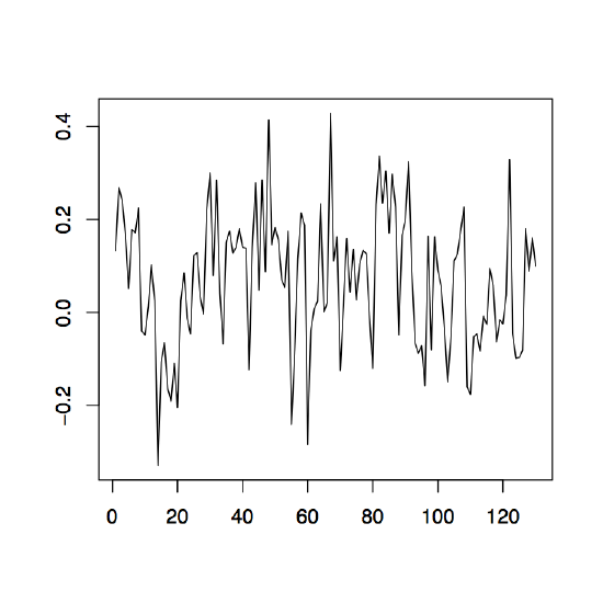
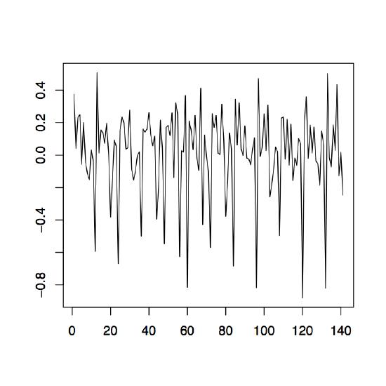
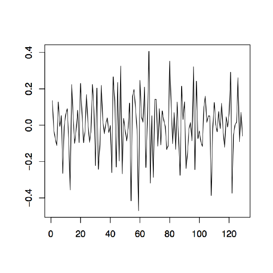
Figure 1.12: The differenced observed series \(\nabla_{12}x_t\) (left), \(\nabla x_t\) (middle) and \(\nabla\nabla_{12}x_t=\nabla_{12}\nabla x_t\) (right) for the Australian red wine sales data.
Example 1.4.2 (Australian wine sales). Revisit the Australian red wine sales data of Example 1.4.1 and apply the differencing techniques just established. The left plot of Figure 1.12 shows the the data after an application of the operator \(\nabla_{12}\). If the remaining trend in the data is estimated with the differencing method from Section 1.3, the residual plot given in the right panel of Figure 1.12 is obtained. Note that the order of application does not change the residuals, that is, \(\nabla\nabla_{12}x_t=\nabla_{12}\nabla x_t\). The middle panel of Figure 1.12 displays the differenced data which still contains the seasonal component.


