7.2: Completely Randomized Design

After identifying the experimental unit and the number of replications that will be used, the next step is to assign the treatments (i.e. factor levels or factor level combinations) to experimental units.

In a completely randomized design, treatments are assigned to experimental units at random. This is typically done by listing the treatments and assigning a random number to each.

In the greenhouse experiment discussed in Chapter 1, there was a single factor (fertilizer) with 4 levels (i.e. 4 treatments), six replications, and a total of 24 experimental units (each unit a potted plant). Suppose the image below is the Greenhouse Floor plan and bench that was used for the experiment (as viewed from above).

Figure \(\PageIndex{1}\): Greenhouse floor plan, showing arrangement of the 24 plants.

We need to be able to randomly assign each of the treatment levels to 6 potted plants. To do this, assign physical position numbers on the bench for placing the pots.

Figure \(\PageIndex{2}\): Greenhouse floor plan, with the plant locations numbered in a grid pattern.

Using Technology

Minitab Example

Steps in Minitab

In Minitab, this assignment can be done by manually creating two columns: one with each treatment level repeated 6 times (order not important) and the other with a position number 1 to \(N\), where \(N\) is the total number of experimental units to be used (i.e. \(N=24\) in this example). The third column will store the treatment assignment.

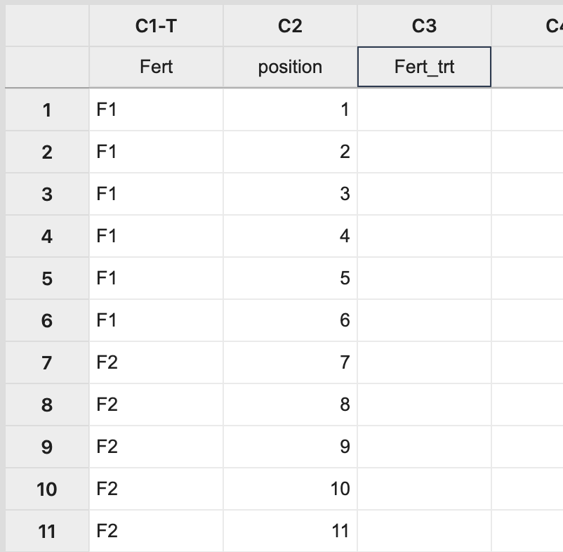
Figure \(\PageIndex{a1}\): Entering treatments, position, and treatment assignment information in Minitab.

Next, select Calc > Sample from Columns, fill in the dialog box as seen below, and click OK.

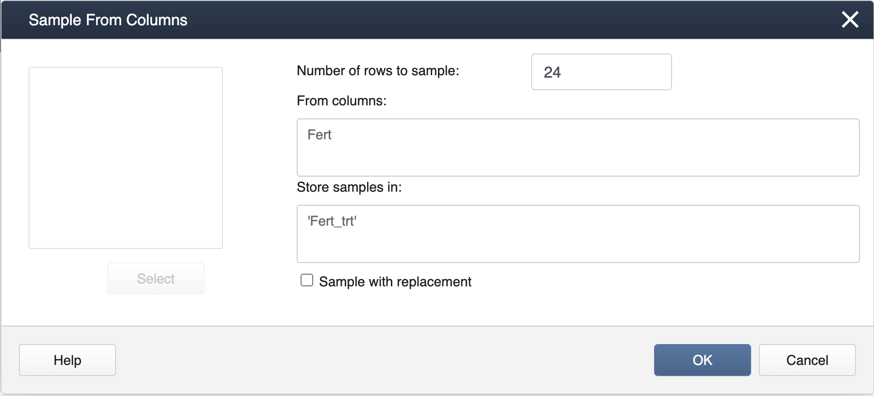
Figure \(\PageIndex{a2}\): Minitab Sample from Columns pop-up window.

Note!

Be sure to have the "Sample with Replacement" box unchecked so that all treatment levels will be assigned to the same number of pots, giving rise to a proper completely randomized design for a specified number of replicates.

This will result in a completely random assignment.

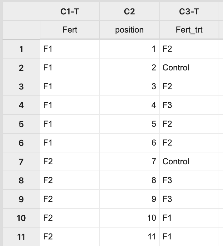
Figure \(\PageIndex{a3}\): Minitab spreadsheet showing the random treatment assignment for each plant position.

This assignment can then be used to apply the treatment levels appropriately to pots on the greenhouse bench.

Figure \(\PageIndex{a4}\): Plants in the greenhouse with their appropriate randomly assigned fertilizer treatment levels.

SAS Example

Steps in SAS

To make the assignments in SAS we can utilize the SAS surveyselect procedure as below:

proc surveyselect data=greenhouse out=trtassignment outrandom
method=srs
samprate=1;
run;

The output would be as below. In practice, it is recommended to specify a seed to ensure the results are reproducible.

Obs	Fertilizer
1	F3
2	F2
3	Con
4	F2
5	F3
6	Con
7	F2
8	F2
9	F3
10	F1
11	F1
12	F3
13	F2
14	F1
15	F3
16	F3
17	F1
18	Con
19	Con
20	F2
21	Con
22	F1
23	Con
24	F1

R Example

Steps in R

Completely Randomized Design

To randomly assign treatment levels to each of our plants we can use the following commands:

sample(treatment)
[1] "F3"      "F2"      "F1"      "F2"      "F3"      "F1"      "Control" "F2"      "F3"     
[10] "F3"      "F2"      "Control" "F3"      "F1"      "F1"      "F2"      "Control" "F2"     
[19] "F1"      "Control" "F3"      "Control" "Control" "F1"     

This means that the first experimental unit will get Fertilizer 3, the second experimental unit will get Fertilizer 2, etc.

Randomized Complete Block Design

Obtain the block design. Load the greenhouse data and obtain the ANOVA table.

To obtain the block design we can use the following commands:

library(blocksdesign)
block_design<-blocks(4,6,6)$Design
obs<-c(1:24)
block<-block_design[,1]
plant<-rep(c(1:4),6)
treatment<-block_design[,3]
data.frame(cbind(obs,block,plant,treatment))
#    obs block plant treatment
# 1    1     1     1         4
# 2    2     1     2         1
# 3    3     1     3         3
# 4    4     1     4         2
# 5    5     2     1         1
# 6    6     2     2         4
# 7    7     2     3         3
# 8    8     2     4         2
# 9    9     3     1         3
# 10  10     3     2         1
# 11  11     3     3         4
# 12  12     3     4         2
# 13  13     4     1         1
# 14  14     4     2         4
# 15  15     4     3         2
# 16  16     4     4         3
# 17  17     5     1         3
# 18  18     5     2         2
# 19  19     5     3         1
# 20  20     5     4         4
# 21  21     6     1         2
# 22  22     6     2         1
# 23  23     6     3         4
# 24  24     6     4         3

To load the greenhouse data and obtain the ANOVA table (lmer() and aov()) we use the following commands:

setwd("~/path-to-folder/")
greenhouse_RCBD_data <- read.table("greenhouse_RCBD_data.txt",header=T)
attach(greenhouse_RCBD_data)
library(lmerTest)
library(lme4)
greenhouse_RCBD_anova<-lmer(Height ~ Fertilizer + (1 | factor(Block)),greenhouse_RCBD_data)
anova(greenhouse_RCBD_anova)
#Type III Analysis of Variance Table with Satterthwaites method
#           Sum Sq Mean Sq NumDF DenDF F value    Pr(>F)    
#Fertilizer 251.44  83.813     3    15  162.96 1.144e-11 ***
#---
#Signif. codes:  0 ‘***’ 0.001 ‘**’ 0.01 ‘*’ 0.05 ‘.’ 0.1 ‘ ’ 1
greenhouse_RCBD_anova1<-aov(Height~Fertilizer+Error(factor(Block)),greenhouse_RCBD_data)
summary(greenhouse_RCBD_anova1)
#Error: factor(Block)
#          Df Sum Sq Mean Sq F value Pr(>F)
#Residuals  5  53.32   10.66               
#Error: Within
#           Df Sum Sq Mean Sq F value   Pr(>F)    
#Fertilizer  3 251.44   83.81     163 1.14e-11 ***
#Residuals  15   7.72    0.51                     
#---
#Signif. codes:  0 ‘***’ 0.001 ‘**’ 0.01 ‘*’ 0.05 ‘.’ 0.1 ‘ ’ 1

For comparison the ANOVA table for the completely randomized design is given below:

greenhouse_CRD_anova<-aov(Height~Fertilizer,greenhouse_RCBD_data)
summary(greenhouse_CRD_anova)
#            Df Sum Sq Mean Sq F value   Pr(>F)    
#Fertilizer   3 251.44   83.81   27.46 2.71e-07 ***
#Residuals   20  61.03    3.05                     
#---
#Signif. codes:  0 ‘***’ 0.001 ‘**’ 0.01 ‘*’ 0.05 ‘.’ 0.1 ‘ ’ 1
detach(greenhouse_RCBD_data)